Data Pipeline for Time Series Data
Table of Contents
- Table of Contents
- Overview: Building a Scalable Time Series Data Pipeline
- Pipeline Orchestration: Streamlining Data Pipeline Management with Airflow on Docker
- Data Ingestion
- AWS Lambda: ETL Job
- AWS Timestream: Time Series Data Warehouse
- Forecasting US Inflation with Temporal Fusion Transformer DNN
Overview: Building a Scalable Time Series Data Pipeline
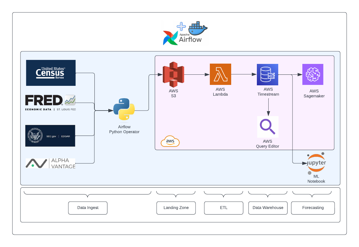
This project involved designing and implementing a robust data pipeline that collects monthly time series data from multiple sources, including FRED, US Census, AlphaVantage, and SEC Edgar, utilizing their respective APIs. Airflow, running within a Docker container, orchestrates the pipeline’s logic as a single DAG. A Python operator within the DAG extracts data from each API and stores it in CSV format within an S3 bucket acting as a data lake/landing zone. The pipeline guarantees the rate limit for each API is respected by limiting Airflow’s maximum parallelism. After the data is stored within the S3 bucket, a Lambda ETL task is initiated to read CSV files, apply necessary transformations, and upload the data to AWS Timestream data warehouse. Users can query time series data effortlessly utilizing SQL queries written on the AWS Query Editor. Moreover, we created a Temporal Fusion Transformer (TFT) model, which predicts inflation (CPI) in the US. This model is deployed on a local Jupyter notebook leveraging CUDA and can also be deployed on a SageMaker instance, enabling continuous data ingestion and prediction.

Pipeline Orchestration: Streamlining Data Pipeline Management with Airflow on Docker
For orchestration, Airflow is a popular open-source platform for managing data pipelines. Its modular and scalable architecture allows users to easily manage and schedule complex workflows. Airflow provides a rich set of built-in operators and plugins for interfacing with a wide variety of data sources and destinations, making it a versatile tool for ETL and general data processing pipelines. Additionally, Airflow’s web interface makes it easy to monitor and troubleshoot pipeline execution. However, Airflow can be complex to set up and configure, and scaling horizontally may require additional infrastructure resources. Additionally, users may need to develop custom operators or plugins to interface with certain data sources or destinations.
Setting up Airflow on Docker
Steps to setup airflow in docker:
- Install Docker Community Edition (CE)
- Install Docker Compose v1.29.1 or newer
- run the following command to fetch the docker-compose.yaml file in terminal:
curl -LfO 'https://airflow.apache.org/docs/apache-airflow/2.6.0/docker-compose.yaml'
- Next, we must extend the official docker image in order to import our python dependencies. First, create a requirements.txt file and import the follwing packages:
apache-airflow[amazon] apache-airflow-providers-http apache-airflow-providers-amazon matplotlib fredapi boto3 setuptools awswrangler cryptography - Now, create a Dockerfile, and add the follwing code to the file:
FROM apache/airflow:2.5.3 COPY requirements.txt /requirements.txt RUN pip install --user --upgrade pip RUN pip install --no-cache-dir --user -r /requirements.txt - Next run the follwing command in terminal:
docker build . --tag extending_airflow:latest
- In the docker-compose.yml, under the webserver section, update image to:
webserver: image: extending_airflow:latest - Now you can simply run/shutdown the docker container using the follwoing commands
docker-compose up -ddocker-compose down
- The default username/password is ‘airflow’, and the airflow ui can be accessed here: http://localhost:4000/fred-data-pipeline/
Data Ingestion
We implemented separate Python operators to collect time series data from various APIs. These operators can be executed sequentially or in parallel to efficiently fetch and process the data. Currently, we are running this pipeline locally since it’s a small task. However, to scale this pipeline, we can leverage the modular architecture of Airflow to run these operators across multiple nodes in a distributed system. This can help improve pipeline throughput and reduce the overall execution time.
Data Sources
We are gathering monthly time series data that pertains to demographic and economic factors. Our data sources include FRED, US Census, alphavantage, and SEC Edgar. The data we are collecting covers a range of economic indicators such as inflation rate, industrial production index, consumer price index, housing starts, crude oil prices, and employment data. In particular, we are focusing on selecting leading indicators that have the potential to provide valuable information on future economic trends, specifically inflation.
Airflow DAG Setup
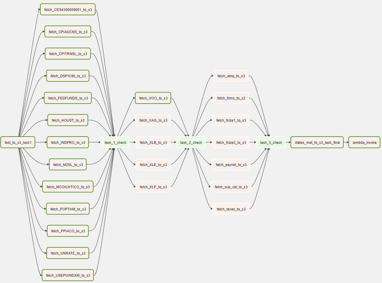
We have implemented separate python_callable files for each data source, which interact with their respective APIs, convert JSON responses to intermediate pandas dataframes, and write them to a CSV file in an S3 bucket. To avoid exceeding API rate limits (set to 10), we utilize Airflow pools. These python_callable tasks may be executed in parallel, but for visual purposes, we run them sequentially as shown in the image below. Following every parallel execution of python operators, a task_#_check is called, which is a dummyoperator. This is necessary because Airflow does not permit [task_list] » [task_list] notation. Instead, we must use [task_list] » dummyOperator » [task_list]. Finally, the lambda ETL job is triggered once all CSV files are written to the S3 bucket.
The following code is for the python_callable for retrieving data from the third party API (AlphaVantage):
        import sys
        import pandas as pd
        from datetime import datetime
        sys.path.append('/opt/airflow/dags/common_package/')
        import config
        from fredapi import Fred
        import awswrangler as wr
        import boto3
        from cryptography.fernet import Fernet
        from airflow.models import Variable
        import requests


        # Define the AWS credentials and S3 bucket name
        #aws_access_key_id = config.get_aws_key_id()
        #aws_secret_access_key = config.get_secret_access_key()
        s3_bucket_name = config.get_s3_bucket()
        fernet_key = config.get_fernet_key()
        fred_api_key = config.get_fred_key()
        vantage_api_key = config.get_alpha_vantage_key()

        # Retrieve the encrypted credentials from Airflow Variables
        encrypted_access_key_id = Variable.get('aws_access_key_id', deserialize_json=False)
        encrypted_secret_access_key = Variable.get('aws_secret_access_key', deserialize_json=False)

        # Decrypt the credentials using the encryption key
        key = fernet_key  # Replace with the encryption key generated in step 1
        fernet = Fernet(key)
        aws_access_key_id = fernet.decrypt(encrypted_access_key_id.encode()).decode()
        aws_secret_access_key = fernet.decrypt(encrypted_secret_access_key.encode()).decode()


        # Define a function to fetch data for a given FRED series and store it in a CSV file in S3
        def fetch_vantage_series_to_s3(vantage_series_id, **context):
            # Make API call and convert fron pd series to dataframe
            vantage_series = get_vantage_series(vantage_series_id, "TIME_SERIES_MONTHLY", vantage_api_key)

            for i in range(2):
                df = vantage_series[i]
                df = df.to_frame().reset_index()
                df = df.rename(columns={0:'value'})

                s3_session = boto3.Session(aws_access_key_id=aws_access_key_id,
                                    aws_secret_access_key=aws_secret_access_key)

                if i == 0: # for close price
                    # Generate a unique file name for the CSV file
                    file_name = f'{vantage_series_id.replace("/", "-")}-{datetime.now().strftime("%Y%m%d")}.csv'
                    # Write the DataFrame to a CSV file and upload it to S3
                    wr.s3.to_csv(df=df, path=f"s3://{s3_bucket_name}/csv-series-vantage/{file_name}", index=False, boto3_session=s3_session)
                else: # for volumne
                    # Generate a unique file name for the CSV file
                    name = f'{vantage_series_id}VOL'
                    file_name = f'{name.replace("/", "-")}-{datetime.now().strftime("%Y%m%d")}.csv'
                    # Write the DataFrame to a CSV file and upload it to S3
                    wr.s3.to_csv(df=df, path=f"s3://{s3_bucket_name}/csv-series-vantage/{file_name}", index=False, boto3_session=s3_session)


        def get_vantage_series(series, function, alpha_vantage_key):
            if function == "TIME_SERIES_MONTHLY":
                url = f"https://www.alphavantage.co/query?function=TIME_SERIES_MONTHLY&symbol={series}&apikey={alpha_vantage_key}"
                r = requests.get(url)
                json_data = r.json()
                monthly_data = json_data["Monthly Time Series"]
                close_series = pd.Series(
                    {datetime.strptime(date, '%Y-%m-%d').replace(day=1): float(data["4. close"]) for date, data in monthly_data.items()},
                    name="Close")
                # Convert the index to a DatetimeIndex
                #print(type(close_series.index))
                #atetime_object = datetime.strptime(str(close_series.index), '%y-%m-%d').replace(day=1)
                #print(datetime_object)
                close_series.index = pd.to_datetime(close_series.index)

                vol_series = pd.Series(
                    {datetime.strptime(date, '%Y-%m-%d').replace(day=1): float(data["5. volume"]) for date, data in monthly_data.items()},
                    name="Volume")
                vol_series.index = pd.to_datetime(vol_series.index)


                close_series.name = series
                vol_series.name = series + "-VOL"

                #close_series.name = close_series.index.replace(day="01")
                #vol_series.name = vol_series.index.replace(day="01")

                data = [close_series, vol_series]
            elif function == "DIGITAL_CURRENCY_MONTHLY":
                url = f'https://www.alphavantage.co/query?function=DIGITAL_CURRENCY_MONTHLY&symbol={series}&market=USD&apikey={alpha_vantage_key}'
                r = requests.get(url)
                json_data = r.json()
                #data = json_data
                monthly_data = json_data["Time Series (Digital Currency Monthly)"]
                close_series = pd.Series(
                    {datetime.strptime(date, '%Y-%m-%d').replace(day=1): float(data["4a. close (USD)"]) for date, data in monthly_data.items()},
                    name="Close")
                # Convert the index to a DatetimeIndex
                print(type(close_series.index))
                close_series.index = pd.to_datetime(close_series.index)

                vol_series = pd.Series(
                    {datetime.strptime(date, '%Y-%m-%d').replace(day=1): float(data['5. volume']) for date, data in monthly_data.items()},
                    name="Volume")
                vol_series.index = pd.to_datetime(vol_series.index)
                data = [close_series, vol_series]
            return data
The code for our dag is shown below.
          from datetime import datetime
          import requests
          import datetime
          from airflow import DAG
          from airflow.operators.python_operator import PythonOperator
          from airflow.operators.dummy_operator import DummyOperator
          from airflow.hooks.S3_hook import S3Hook


          import sys
          sys.path.append('/opt/airflow/dags/common_package/')
          import config
          import fetch_fred_series_s3
          import states_met_to_s3
          import lambda_invoke
          import fetch_vantage_series_s3
          import fetch_census_series_s3

          def test_task():
            print("First dag task test: successful")

          # Define the DAG
          # to limit the number of proccess calling fred api (60/min) ~ we limit the execution parallelism to 10 tasks using airflow pools
          with DAG(
              'fred_to_s3_batch_dag',
              start_date=datetime.datetime(2023, 4, 10),
              schedule_interval='@once', #Batch upload
              catchup=False,
              default_args={
                  'owner': 'airflow',
                  'depends_on_past': False,
                  'email_on_failure': False,
                  'email_on_retry': False,
                  'retries': 2,
                  'retry_delay': datetime.timedelta(minutes=5),
                  'pool':'fred_batch_pool'
              }
          ) as dag:

            test_task1 = PythonOperator(
              task_id='test_to_s3_task1',
              python_callable=test_task,
            )


            states_met_to_s3_task_final = PythonOperator(
              task_id='states_met_to_s3_task_final',
              python_callable=states_met_to_s3.states_met_to_s3,
              op_kwargs={
                  'test': 'Last time this works',
              },
              provide_context=True,
            )

            lambda_invoke = PythonOperator(
              task_id='lambda_invoke',
              python_callable=lambda_invoke.lambda_invoke_test
            )

            task_1_check = DummyOperator(task_id='task_1_check')

            task_2_check = DummyOperator(task_id='task_2_check')

            task_3_check = DummyOperator(task_id='task_3_check')


          # Define a list of FRED series IDs to fetch
          fred_series_ids = ["CPIAUCNS", # Target

                        "M2SL", "INDPRO", "PPIACO", "CPITRNSL", "POPTHM", "CES4300000001", "USEPUINDXM", "DSPIC96", # CONVERT TO GROWTH RATE

                        "HOUST", "MCOILWTICO", "FEDFUNDS", "UNRATE" # Keep as is
                      ]
          # Define a PythonOperator for each FRED series to fetch
          fred_series_tasks = []
          for fred_series_id in fred_series_ids:
              task_id = f'fetch_{fred_series_id}_to_s3'
              op = PythonOperator(
                  task_id=task_id,
                  python_callable=fetch_fred_series_s3.fetch_fred_series_to_s3,
                  op_kwargs={
                      'fred_series_id': fred_series_id,
                  },
                  provide_context=True

              )
              fred_series_tasks.append(op)


          vantage_series_ids = ["VOO", "XLP", "XLE", "XLB", "XAG"] # voo = market trackings, xlp=consumer staples, xle = energy, xlb = basic materials, xag = gold
          vantage_series_tasks = []
          for vantage_series_id in vantage_series_ids:
              task_id_vantage = f'fetch_{vantage_series_id}_to_s3'
              op = PythonOperator(
                  task_id=task_id_vantage,
                  python_callable=fetch_vantage_series_s3.fetch_vantage_series_to_s3
          ,
                  op_kwargs={
                      'vantage_series_id': vantage_series_id,
                  },
                  provide_context=True

              )
              vantage_series_tasks.append(op)

          vantage_series_ids = ["VOO"]


          census_series_ids = ["firms", "emp", "fsize1", "fsize2", 'taxes', "payroll", "sup_val"]
          census_series_tasks = []
          for census_series_id in census_series_ids:
              task_id_census = f'fetch_{census_series_id}_to_s3'
              op = PythonOperator(
                  task_id=task_id_census,
                  python_callable=fetch_census_series_s3.fetch_census_series_to_s3
          ,
                  op_kwargs={
                      'series_id': census_series_id,
                  },
                  provide_context=True

              )
              census_series_tasks.append(op)


          # Set the task dependencies so that all FRED series are fetched in parallel
          test_task1  >> fred_series_tasks >> task_1_check >> vantage_series_tasks >> task_2_check >> census_series_tasks >> task_3_check >> states_met_to_s3_task_final >>  lambda_invoke
AWS S3: Landing zone for CSV files
AWS S3 serves as our landing zone for all the CSV files generated by the data ingestion pipeline. We created an S3 bucket in the same region as our Airflow lambda instance for low latency access. This region choice is important as it can affect network latency and data transfer rates. In addition, we enabled versioning on the S3 bucket to ensure we can access previous versions of the CSV files if necessary.
Having a landing zone for our CSV files is an important component of a data pipeline as it allows us to store, access, and process large amounts of data efficiently. This is often referred to as a “data lake” approach, where data is stored in its raw form and processed as needed. An alternative approach is the “ELT” (extract, load, transform) method, where data is extracted from its source, loaded into a centralized database, and then transformed into a usable format. While both approaches have their pros and cons, the data lake approach allows for greater flexibility and scalability as it enables processing of data in its raw form without the need for complex ETL processes.
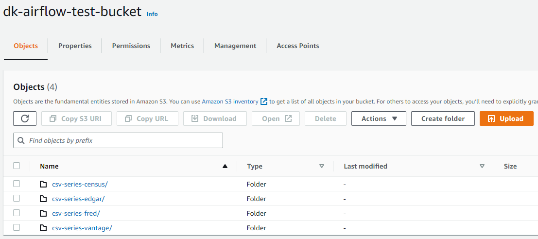
Note that the S3 bucket name must be unique globally. Our bucket is called dk-airflow-test-bucket. Below we can see that a separate folder is created for each of the data sources.
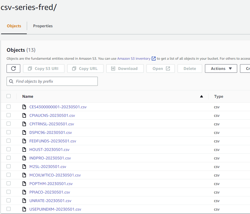
Next, we can see all the files that have been added to the folder for FRED, after a successful DAG run.
AWS Lambda: ETL Job
This ETL (Extract, Transform, Load) job comprises a Python script that functions as an AWS Lambda triggered by Airflow following successful ingestion of data into S3. The job reads and transforms multiple CSV files from an S3 bucket, and then writes the data to Amazon Timestream, a fully managed time series database. Notably, if a Timestream Table already contains data, only missing or future values are inserted into the database. The following are the primary steps of this job:
AWS Lambda Setup
Lambda Setup:
- Memory: 128 MB, Ephemeral Storage: 512 MB, Timeout: 2 min (price per 1ms: $0.0000000083, Free Tier Eligible)
- We add a layer to our lambda function to allow us to work with pandas (arn:aws:lambda:us-east-2:336392948345:layer:AWSSDKPandas-Python39:6).
- We assign an create an IAM Role with full read/write access to Timestream and S3, and assign it to the lambda function
ETL Overview: Batch Writing to Timestream
ETL Steps:
- Define the S3 bucket, Timestream client, and the database and table names, utilizing the boto3 package for python to communicate with AWS services.
- Create a Timestream table with the create_timestream_table function, as detailed in the (#AWS Timestream Setup) section.
- Extract: Read CSV files from each folder in the S3 bucket and merge them into a single Pandas dataframe through joining on date_index.
- Transform: Convert pandas datetime to Unix timestamp and create a Timestream record if year >= 1970 (or has a non-negative Unix value).
- Load: Batch write to Timestream with a batch size of 100 Timestream records to maximize throughput.
The code for this ETL job is displayed below (also on github):
        import json
        import boto3
        import re
        from datetime import datetime, timezone
        import time
        import pandas as pd
        import math


        def lambda_handler(event, context):
            # specify region to be us-east-2 for s3
            s3 = boto3.resource('s3', region_name='us-east-2')
            bucket = s3.Bucket('dk-airflow-test-bucket')
            client = boto3.client('timestream-write', region_name='us-east-2')
            print(client.meta.region_name)
            bucket_name = 'dk-airflow-test-bucket'
            database_name = 'fred-batch-data'
            table_name = 'csv_series_fred_combined'


            create_timestream_table(client, table_name, database_name)

            df = read_s3_csv_multiple(bucket_name, 'csv-series-fred')

            print(df.head())
            print(f'df shape: {df.shape}')

            create_timestream_records_df(client, table_name, database_name, df)

            return "Success"


        def read_s3_csv(bucket, key):
            s3 = boto3.resource('s3', region_name='us-east-2')
            obj = s3.Object(bucket, key)
            return obj.get()['Body'].read().decode('utf-8').split('\n')


        # read multiple csv files from s3 and return a list of lists of rows with date as index


        def read_s3_csv_multiple(bucket, prefix):
            s3 = boto3.resource('s3', region_name='us-east-2')
            csv_list = []

            for obj in s3.Bucket(bucket).objects.all():
                # Get the filename from the object key
                filename = obj.key.split('/')[-1]
                print(f'filename: {filename}')

                # Check if file is CSV and not empty
                if not filename.endswith('.csv') or obj.size == 0:
                    continue

                # Read the CSV file from S3 into a pandas dataframe
                csv_obj = s3.Object(bucket, obj.key)
                body = csv_obj.get()['Body']
                df = pd.read_csv(body, index_col=0, parse_dates=True)

                # Rename the first column to the filename (without extension)
                col_name = filename.split('.')[0]
                df.rename(columns={df.columns[0]: col_name}, inplace=True)

                # Add the dataframe as a new column in the csv_list
                csv_list.append(df.iloc[:, 0])

            # Combine all the dataframes in the csv_list into a single dataframe using the index as the key
            final_df = pd.concat(csv_list, axis=1)

            # Add a new column called "date" with the date index as the values
            final_df['date_index'] = final_df.index

            return final_df


        def create_timestream_table(client, table_name, database_name):
            print('table name: ', table_name)
            try:
                client.create_table(
                    DatabaseName=database_name,
                    TableName=table_name,
                    RetentionProperties={
                        'MemoryStoreRetentionPeriodInHours': 24,
                        'MagneticStoreRetentionPeriodInDays': 73000
                    },
                    Tags=[],
                    MagneticStoreWriteProperties={
                        'EnableMagneticStoreWrites': True,
                        'MagneticStoreRejectedDataLocation': {
                            'S3Configuration': {
                                'BucketName': 'dk-airflow-test-bucket',
                                'ObjectKeyPrefix': 'rejected-data/',
                                'EncryptionOption': 'SSE_S3'
                            }
                        }
                    }
                )
                print(f"Created table {table_name} in database {database_name}")
            except client.exceptions.ValidationException as e:
                print(f"Error creating table {table_name}: {str(e)}")
            except Exception as e:
                print(f"Unknown error creating table {table_name}: {str(e)}")


        def create_timestream_records(client, table_name, database_name, rows):
            records_details = {
                'DatabaseName': database_name,
                'TableName': table_name,
            }

            records = []
            record_counter = 0

            table_name_split = table_name.split('_')

            try:
                series_name = table_name_split[3]
            except ValueError:
                print(table_name_split)
                series_name = table_name


            count = len(rows[1:])
            print(f"row count: {count}")
            for row in rows[1:]:
                values = row.split(',')
                if len(values) != 2:
                    print(f"Error: {row} does not have 2 values (lmd)")
                    print(f"values: {values}")
                    continue

                # Convert timestamp to unix
                try:
                    values[0] = re.sub(r"[-]", "/", values[0])
                    if validate_y_m_d(values[0]) == True:
                        date_obj = datetime.strptime(values[0], '%Y/%m/%d')
                    else:
                        date_obj = datetime.strptime(values[0], '%m/%d/%Y')
                    if date_obj < datetime(1970, 1, 1):
                        continue

                    timestamp = int(date_obj.timestamp() * 1000)
                    #print('entered this')
                except ValueError:
                    #print(f"Invalid date string: {values[0]}")
                    continue


                #print(f'exited after')
                # Create a new record with the current time as the timestamp
                current_time = str(int(round(time.time() * 1000)) - (count))
                #print(f'current time: {current_time}')


                multi_record = {
                    'Dimensions': [
                        {'Name': 'S3 Region', 'Value': 'us-east-2'}
                    ],
                    'MeasureValueType': 'MULTI',
                    'MeasureName': series_name,
                    'Time': current_time,
                    'MeasureValues': [
                    {'Name': 'Date', 'Type': 'TIMESTAMP', 'Value': str(timestamp)},
                    {'Name': 'Value', 'Type': 'DOUBLE', 'Value': str(values[1]) }
                    ]
                }

                records.append(multi_record)
                record_counter += 1
                count += 10

                if len(records) == 100:
                    batch_to_timestream(client, table_name, database_name, records, record_counter)
                    records= []

            if len(records) != 0:
                batch_to_timestream(client, table_name, database_name, records, record_counter)

            #print(f"table {table_name}, with {len(records['Records'])} actual records")
            return True


        def create_timestream_records_df(client, table_name, database_name, df):
            records = []
            record_counter = 0
            count = 0

            for index, row in df.iterrows():

                # Check if the date in 'date_index' column is before the Unix time
                if row['date_index'] < datetime(1970, 1, 1):
                  # print(f"Invalid date string: {row['date_index']}")
                    continue

                current_time = str(int(round(time.time() * 1000)) - (record_counter*100))

                # create measure values for each column in the row
                measure_values = []
                for col in df.columns:
                    if col == 'date_index':

                        #ts_date = datetime.strptime(row[col], '%Y-%m-%d %H:%M:%S')
                        ts_date = row[col].to_pydatetime()
                        timestamp = int(ts_date.timestamp() * 1000)
                        print(f'type = {type(row[col])} ,row[col]: {row[col]},  Timestamp: {timestamp}')


                        measure_values.append({'Name': 'date_index', 'Type': 'TIMESTAMP', 'Value': str(timestamp)})


                    else:
                    # Check for NaN values and replace them with null
                        value = row[col]
                        if pd.isna(value):
                            value = str(float(0.0))
                        else:
                            value = str(value)
                        col_name = col.split('-')[0]
                        measure_values.append({'Name': col_name, 'Type': 'DOUBLE', 'Value': value})

                # Create a new record with the current time as the timestamp
                multi_record = {
                    'Dimensions': [
                        {'Name': 'S3 Region', 'Value': 'us-east-2'}
                    ],
                    'MeasureValueType': 'MULTI',
                    'MeasureName': 'fred_pipeline_measure',
                    'Time': current_time,
                    'MeasureValues': measure_values
                }

                records.append(multi_record)
                record_counter += 1

                if len(records) == 100:
                    batch_to_timestream(client, table_name, database_name, records, record_counter)
                    records = []

            if len(records) != 0:
                batch_to_timestream(client, table_name, database_name, records, record_counter)

            return True


        def batch_to_timestream(client, table_name, database_name, records, counter):
            try:
                result = client.write_records(DatabaseName=database_name, TableName=table_name,
                                                    Records=records, CommonAttributes={})
                print("Processed [%d] records. WriteRecords Status: [%s]" % (counter,
                                                                                result['ResponseMetadata']['HTTPStatusCode']))
            except client.exceptions.RejectedRecordsException as err:
                print("RejectedRecords: ", err)
                for rr in err.response["RejectedRecords"]:
                    print("Rejected Index " + str(rr["RecordIndex"]) + ": " + rr["Reason"])
                print("Other records were written successfully. ")
            except Exception as err:
                print("Error:", err)

        def delete_table(client, table_name, database_name):
            print("Deleting Table")
            try:
                result = client.delete_table(DatabaseName=database_name, TableName=table_name)
                print("Delete table status [%s]" % result['ResponseMetadata']
                ['HTTPStatusCode'])
            except client.exceptions.ResourceNotFoundException:
                print("Table [%s] doesn't exist" % table_name)
            except Exception as err:
                print("Delete table failed:", err)


        def validate_y_m_d(date_str):
            pattern = r'^(\d{4})[-/](\d{1,2})[-/](\d{1,2})$'
            match = re.match(pattern, date_str)
            if not match:
                return False
            year, month, day = match.groups()
            year = int(year)
            month = int(month)
            day = int(day)
            try:
                datetime(year, month, day)
                return True
            except ValueError:
                return False
AWS Timestream: Time Series Data Warehouse
AWS Timestream is a fully managed time-series database service offered by Amazon Web Services (AWS) that is designed to handle large-scale time series data with high durability and availability. Unlike traditional SQL databases, Timestream is optimized for handling time series data and provides features like automatic scaling, data retention management, and the ability to query large datasets quickly. One of the main advantages of Timestream over traditional databases is that it allows for efficient and easy storage and retrieval of time series data at scale.
Other populer alternatives to Timstream include InfluxDB, OpenTSDB, and TimescaleDB. These databases provide similar features to Timestream, but they may differ in terms of performance, scalability, and ease of use. InfluxDB, for instance, is a popular open-source time-series database that offers high write and query performance and supports SQL-like query languages. OpenTSDB is another popular open-source database that provides horizontal scaling and advanced features like histograms and percentile aggregations. TimescaleDB is an open-source database that extends PostgreSQL to handle time-series data and provides features like automatic data partitioning and multi-node clustering. However, Timestream is specifically designed and optimized for the AWS ecosystem, which makes it a better choice if you are already using AWS services and need a fully managed time-series database that can easily integrate with other AWS services.
AWS Timestream Setup
Our created Timestream table has the following properties:
- Database retention period: 73000 days for magnetic store (Max amount for historical data) and 24 hours for memory store
- Note: Magnetic Store is for larger volume & cost effective long storage, while memory store is for faster access of recently stored data
- Memory store and magnetic store writes are enabled
- Magnetic store rejected data is stored in an S3 bucket with Server-Side Encryption (SSE-S3)
Forecasting US Inflation with Temporal Fusion Transformer DNN