Forecasting Inflation (CPI) with Temporal Fusion Transformers (TFT)
Table of Contents
- Table of Contents
- Project Overview
- Project Setup
- Data Cleaning/Transformations
- Visualizations
- Temporal Fusion Transformer (TFT) Model
- Additional Feature Engineering
- Load The Data
- Create Baseline Model
- Train the Temporal Fusion Transformer
- Hyperparameter Tuning With Optuna
- Best Model From Optuna Hyperparameter Optimization
Project Overview
Data: The project utilizes economic and demographic time series data collected from various sources, including FRED and AlphaVantage, stored in a table on AWS Timestream. The target variable is the year-over-year growth rate of the Consumer Price Index for All Urban Consumers (CPIAUCNS) from FRED data.
Preprocessing: The series, including the target variable, are transformed into growth rates to satisfy stationarity requirements. Data validation, MinMax scaling, and further feature engineering are performed to capture seasonality and encode special dates. The data is loaded into a TimeSeriesDataSet dataloader, where a look-back window, prediction interval, and training/validation split are defined.
Model: Temporal Fusion Transformers model (TFT) is used for forecasting. TFT is a DNN designed for time series prediction, which combines traditional time series techniques, such as ARIMA and exponential smoothing, with deep learning methods such as LSTMs and Transformers. The model takes in multiple input time series, including the 15 predictors, as well as any relevant external events such as unscheduled FED meetings or recessions. These inputs are first preprocessed to account for seasonality, trends, missing data, and MinMax scaling. The model then uses an attention mechanism to weigh the importance of each input time series and generate a set of fused representations, which are fed into a set of stacked Transformer layers that learn to encode temporal dependencies and generate predictions.
Hyperparameter Optimization: This project utilized Optuna, an open-source hyperparameter optimization framework, to optimize the hyperparameters for our TFT model. We created a study to explore the best hyperparameter configuration for our model by evaluating a set of hyperparameters across multiple trials. We set up the study to run 50 trials, each with a maximum of 75 epochs. We specified a range of values for each of the hyperparameters, including gradient clip value, hidden size, continuous hidden size, attention head size, learning rate, and dropout rate.
Assessment:
Conclusion:
# ADD RESULTS SNEAK PEEK
Project Setup
Imports
# Suppress warnings
import os
import warnings
warnings.filterwarnings("ignore")  # avoid printing out absolute paths
# Plotting Libraries
%matplotlib inline
import matplotlib.pyplot as plt
from IPython.core.pylabtools import figsize
import plotly.express as px
import plotly.offline as pyo
import plotly.io as pio

from ipywidgets import interact, SelectionRangeSlider

# Data transforming / importing
import numpy as np
import pandas as pd
import requests
import io
import time
import config
import boto3
import botocore
import sys
from cryptography.fernet import Fernet
import awswrangler as wr
from datetime import datetime
import copy
from pathlib import Path

# pytorch
import torch

# pytorch-lightning - Hyperparameter optimization
import lightning.pytorch as pl
from lightning.pytorch.callbacks import EarlyStopping, LearningRateMonitor
from lightning.pytorch.loggers import TensorBoardLogger
import tensorboard
import tensorboardX
from tqdm.notebook import tqdm

# pytorch-forecasting
from pytorch_forecasting import Baseline, TemporalFusionTransformer, TimeSeriesDataSet
from pytorch_forecasting.data import EncoderNormalizer
from pytorch_forecasting.metrics import RMSE, MAE, SMAPE, PoissonLoss, QuantileLoss, DistributionLoss, MultivariateDistributionLoss
from pytorch_forecasting.models.temporal_fusion_transformer.tuning import optimize_hyperparameters
from sklearn.preprocessing import MinMaxScaler
Retrieve Credentials
# Define the AWS credentials and S3 bucket name
s3_bucket_name = config.get_s3_bucket()
fernet_key = config.get_fernet_key()
fred_api_key = config.get_fred_key()
alpha_vantage_key = config.get_alpha_vantage_key()

# Retrieve the encrypted credentials
encrypted_access_key_id = config.get_encrypted_aws_key_id()
encrypted_secret_access_key = config.get_encrypted_secret_access_key()

# Decrypt the credentials using the encryption key
key = fernet_key
fernet = Fernet(key)
aws_access_key_id = fernet.decrypt(encrypted_access_key_id.encode()).decode()
aws_secret_access_key = fernet.decrypt(encrypted_secret_access_key.encode()).decode()
ENDPOINT = 'us-east-2' # <--- specify the location for timestream db
PROFILE = "default" # <--- specify the AWS credentials profile
DB_NAME = "fred-batch-data" # <--- specify the database created in Amazon Timestream
TABLE_NAME = "csv_series_fred_combined" # <--- specify the table created in Amazon Timestream

# Create AWS boto3 session
s3_session = boto3.Session(aws_access_key_id=aws_access_key_id,
                    aws_secret_access_key=aws_secret_access_key)
Retrieve data from AWS Timestream Database
- To retrieve data from the AWS Timestream database, we can use SQL queries with the aws wrangler library.
- The data we are retrieving was collected for the fred-pipeline project and has the following properties:
- Monthly timeseries data
- Collected from 1970 to present
- Sources
- FRED (Federal Reserve Economic Data)
- AlphaVantage (a third-party API for stock, cryptocurrency, and economic data)
- US Census Bureau
# sql query to retireve all data from our combined fred database
query = f'SELECT * FROM "{DB_NAME}"."{TABLE_NAME}"'
original_df = wr.timestream.query(query, boto3_session=s3_session)
df = original_df.copy()
Data Cleaning/Transformations
The following steps describe the process for transforming and cleaning our pandas DataFrame:
-
Convert the date_index column from a string to a datetime object and set it as the DataFrame’s index. The DataFrame is then sorted in ascending order by the index.
-
Transform a list of series IDs by calculating the percentage change in growth rate over the previous 12 months, storing the result in a new column in the DataFrame with the “_GR” suffix, and dropping the original column for each series.
-
Remove the first 12 rows and the last 2 rows from the DataFrame, as the growth rate will be NaN for the first 12 months and the last 2 rows may contain missing data.
-
Remove any remaining non-numeric columns from the DataFrame.
-
Mean-normalize the DataFrame by subtracting the mean from each value and dividing by the standard deviation. The resulting DataFrame is named normalized_df and will be used to create data exploration visuals. (Only used for visualization)
# Convert date index from string to datetime and set it to index
df['date_index'] = pd.to_datetime(df['date_index'])
df.set_index('date_index', inplace=True)
df = df.sort_index()
series_ids_to_gr = ["CPIAUCNS", # Target
              "M2SL", "INDPRO", "PPIACO", "CPITRNSL", "POPTHM", "DSPIC96"]

# Retrieve series form fred and convert to growth rate, delete original cols
for series in series_ids_to_gr:
    df_growth = df[series].pct_change(12) * 100 # GROWTH RATE PREVIOUS YEAR SAME PERIOD
    df[f"{series}_GR"]= df_growth
    df.pop(series)
# drop first 12 rows (as growth rate will be NaN for first 12 months)
# drop last 2 rows as NaN due to missing data
df = df[12:-2]
df = df.fillna(0)
df.tail()
| S3 Region | measure_name | time | VOOVOL | USEPUINDXM | UNRATE | FEDFUNDS | HOUST | CES4300000001 | VOO | MCOILWTICO | CPIAUCNS_GR | M2SL_GR | INDPRO_GR | PPIACO_GR | CPITRNSL_GR | POPTHM_GR | DSPIC96_GR | |
|---|---|---|---|---|---|---|---|---|---|---|---|---|---|---|---|---|---|---|
| date_index | ||||||||||||||||||
| 2022-10-01 | us-east-2 | fred_pipeline_measure | 2023-05-01 16:14:49.658 | 99172672.0 | 177.42313 | 3.7 | 3.08 | 1426.0 | 6741.7 | 354.95 | 87.55 | 7.745427 | 1.493661 | 3.097468 | 10.228516 | 11.243300 | 0.435538 | -1.993596 |
| 2022-11-01 | us-east-2 | fred_pipeline_measure | 2023-05-01 16:14:49.558 | 78860409.0 | 171.73726 | 3.6 | 3.78 | 1419.0 | 6704.6 | 374.49 | 84.37 | 7.110323 | 0.379527 | 1.852622 | 8.167309 | 7.863496 | 0.449833 | -1.354907 |
| 2022-12-01 | us-east-2 | fred_pipeline_measure | 2023-05-01 16:14:49.458 | 94164717.0 | 136.43315 | 3.5 | 4.10 | 1348.0 | 6704.9 | 351.34 | 76.44 | 6.454401 | -0.893723 | 0.584918 | 6.871276 | 3.708271 | 0.463836 | -0.751117 |
| 2023-01-01 | us-east-2 | fred_pipeline_measure | 2023-05-01 16:14:49.359 | 76631756.0 | 143.09753 | 3.4 | 4.33 | 1334.0 | 6736.6 | 373.44 | 78.12 | 6.410147 | -1.622770 | 1.388797 | 5.583215 | 3.602555 | 0.485104 | 2.993189 |
| 2023-02-01 | us-east-2 | fred_pipeline_measure | 2023-05-01 16:14:49.259 | 70631595.0 | 124.15729 | 3.6 | 4.57 | 1432.0 | 6716.1 | 364.11 | 76.83 | 6.035613 | -2.294358 | 0.946530 | 2.389377 | 2.447774 | 0.503966 | 3.238219 |
# Remove all non numeric columns
numerics = ['int16', 'int32', 'int64', 'float16', 'float32', 'float64']
clean_df = df.select_dtypes(include=numerics)
# mean normalized dataframe
normalized_df=(clean_df-clean_df.mean())/clean_df.std()
normalized_df.tail()
| VOOVOL | USEPUINDXM | UNRATE | FEDFUNDS | HOUST | CES4300000001 | VOO | MCOILWTICO | CPIAUCNS_GR | M2SL_GR | INDPRO_GR | PPIACO_GR | CPITRNSL_GR | POPTHM_GR | DSPIC96_GR | |
|---|---|---|---|---|---|---|---|---|---|---|---|---|---|---|---|
| date_index | |||||||||||||||
| 2022-10-01 | 2.838965 | 1.517436 | -1.469023 | -0.448885 | -0.025206 | 2.592309 | 2.877923 | 1.679542 | 1.253909 | -1.465478 | 0.217776 | 1.015321 | 1.196767 | -2.117406 | -1.744359 |
| 2022-11-01 | 2.170538 | 1.424803 | -1.528045 | -0.272349 | -0.041962 | 2.558916 | 3.062945 | 1.581789 | 1.040748 | -1.753379 | -0.045225 | 0.677413 | 0.637394 | -2.057261 | -1.512745 |
| 2022-12-01 | 2.674165 | 0.849637 | -1.587066 | -0.191647 | -0.211913 | 2.559186 | 2.843741 | 1.338021 | 0.820599 | -2.082397 | -0.313056 | 0.464945 | -0.050315 | -1.998345 | -1.293786 |
| 2023-01-01 | 2.097198 | 0.958211 | -1.646087 | -0.133643 | -0.245424 | 2.587719 | 3.053003 | 1.389664 | 0.805746 | -2.270788 | -0.143218 | 0.253784 | -0.067811 | -1.908863 | 0.064050 |
| 2023-02-01 | 1.899747 | 0.649642 | -1.528045 | -0.073116 | -0.010844 | 2.569267 | 2.964658 | 1.350010 | 0.680040 | -2.444332 | -0.236657 | -0.269805 | -0.258933 | -1.829507 | 0.152908 |
Visualizations
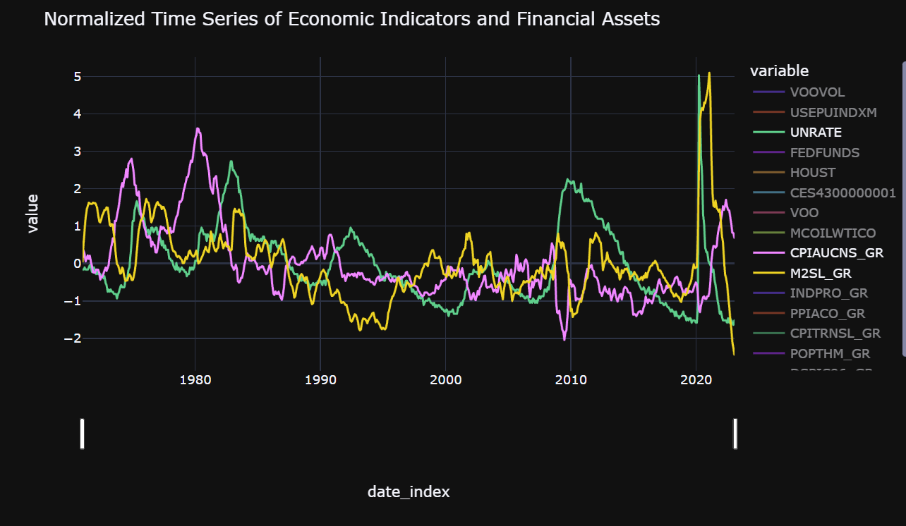
Figure 1: Comparison of Monthly Time Series Data
We have created our visualizations using Plotly Express. The visualization is interactive, and you can select or deselect specific series from the variable section. Additionally, you can adjust the date range using the slider at the bottom of the visual.
The default visualization displays the following series:
- CPIAUCNS_GR: Consumer Price Index for All Urban Consumers: All Items in U.S. City Average (Target variable, converted to growth rate)
- UNRATE: Unemployment Rate
- M2SL_GR: M2 money stock converted to growth rate
You can customize the visual to display additional time series data as per your requirement.
series_to_hide = ["INDPRO_GR", "PPIACO_GR", "CPITRNSL_GR", "POPTHM_GR", "DSPIC96_GR",  # GROWTH RATES
                "HOUST", "MCOILWTICO", "FEDFUNDS", "VOO", "VOOVOL", "USEPUINDXM", "CES4300000001"]
fig = px.line(normalized_df, x = normalized_df.index, y = normalized_df.columns, template = 'plotly_dark')
fig.update_xaxes(rangeslider_visible=True)

fig.for_each_trace(lambda trace: trace.update(visible="legendonly")
                   if trace.name in series_to_hide else ())
# Generate the HTML rendering of the plot using Plotly IO
#html = pio.to_html(fig, include_plotlyjs=False)
pio.write_html(fig, file='fig1_vis.html')

fig.show()
# Display the HTML rendering of the plot
#pyo.iplot(html)
Figure 2: Correlation Heatmap of Mean-Normalized Data
We have used Plotly Express to create an interactive heatmap of the correlation matrix of the mean-normalized data.
The color scale in the heatmap represents the correlation coefficients between -1 and 1, where -1 indicates a perfect negative correlation, 0 indicates no correlation, and 1 indicates a perfect positive correlation. The closer the coefficient is to 1 or -1, the stronger the correlation between the two variables.
The following series have the strongest correlation with our target “CPIAUNS_GR”:
- PPIACO_GR: Producer Price Index - PPI (0.75 ~ Positive correlation)
- Article by the Richmond Fed found evidence that their model found evidence that the two price indexes move together over the long run — a relationship that economists call cointegration (PPI & CPI)
- Link To FED Article.
- FEDFUNDS: Federal Funds Rate (0.69 ~ Positive Correlation)
- This rate is adjusted by the Fed according to the economic conditions and used as a tool to combat high inflation (higher fedfunds rate implies a more aggressive response to inflation).
- USEPUINDXM: Economic Policy Uncertainty Index (-0.57 ~ Negative Correlation)
- Higher economic uncertainty often leads to less consumer/business spending which could lead to lower prices due to falling demand.
fig2 = px.imshow(normalized_df.corr(), template = 'plotly_dark')

pio.write_html(fig2, file='fig2_vis.html')
# Display the HTML rendering of the plot
#pyo.iplot(html2)

fig2.show()
Temporal Fusion Transformer (TFT) Model
-
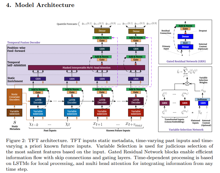
Temporal Fusion Transformers (TFT) are a type of neural network designed for time series prediction. It combines traditional time series techniques (such as ARIMA and exponential smoothing) with deep learning methods (such as LSTMs and Transformers).
-
Our model takes in multiple input time series, including the 15 predictors as well as any relevant external events (such as unscheduled FED meetings or recessions). The inputs are first preprocessed to account for seasonality, trends, missing data, and minmax scaled.
-
The model then uses an attention mechanism to weigh the importance of each input time series and generate a set of fused representations. These representations are fed into a set of stacked Transformer layers, which learn to encode temporal dependencies and generate predictions. The model can be trained using a variety of loss functions, such as mean squared error or mean absolute error. Our model uses quantile loss, which provides a prediction distribution in additon to a simple prediction.
Temporal Fusion Transformer (TFT) Architecture Overview
-
Inputs: The model takes in static metadata (e.g. categorical features), time-varying past inputs (e.g. previous values of CPIAUCNS_GR), and time-varying future inputs (e.g. FRED economic indicators).
-
Embeddings: Each input is transformed into a high-dimensional embedding vector, which is used to capture non-linear relationships between the inputs.
-
Encoding: The embedded inputs are then fed into a set of LSTM encoder layers, which learn to encode the temporal dependencies between the inputs.
-
Decoding: The LSTM encoder output is passed through a set of self-attention Transformer decoder layers, which learns to generate future predictions by attending to the relevant inputs.
-
Fusion: The Transformer decoder generates a set of fused representations that are used to weight the importance of each input time series.
-
Prediction: The fused representations are fed through a set of fully connected layers, which produce the final prediction. The model is trained using a quantile loss function, which provides a probabilistic estimate of the predicted value.
-
Hierarchical: The model is trained using a hierarchical training approach, where the outputs of the lower-level models are used as inputs to the higher-level models. This allows the model to capture multiple levels of temporal dependencies and generate accurate long-term predictions.
TFT Strengths
-
Highly flexible and can handle time series data with different scales and frequencies, and incorporate exogenous variables.
-
Suitable for various forecasting tasks, from short-term to long-term predictions, and can be used in different industries such as finance, energy, and healthcare.
-
The attention mechanism enables the model to capture complex patterns and relationships in the data, improving its accuracy compared to simpler models such as autoregressive models.
-
Can handle special events or holidays as exogenous inputs, allowing the model to capture the impact of such events on the time series data.
TFT Shortcomings
-
The model’s computational complexity can make it challenging to train on large datasets.
-
The model’s architecture is composed of several multi-head attention and feedforward neural network layers, leading to slow training times and requiring significant computational resources.
-
The model’s reliance on past values to make future predictions may not be suitable for forecasting scenarios where the future may be influenced by factors that are not captured by historical data, such as sudden changes in external conditions or the introduction of new variables.
-
The model’s assumption of stationary data can limit its applicability to non-stationary time series data.
# deal with cuda memory issues
torch.cuda.empty_cache()
Additional Feature Engineering
- Validate our dataframe (check if any of the columns contains NA/inf values)
- MinMax scale our dataframe (using scikit learn MinMaxScaler() functions)
- Encode special days as one variable and thus use reverse one-hot encoding. Special days includes dates/date ranges for recessions (post 1970) and unscheduled fed (FOMC) meetings
- Add time based features to capture seasonality (day, month, year)
clean_df.replace([np.inf, -np.inf], np.nan, inplace=True)
clean_df.isna().any()
VOOVOL           False
USEPUINDXM       False
UNRATE           False
FEDFUNDS         False
HOUST            False
CES4300000001    False
VOO              False
MCOILWTICO       False
CPIAUCNS_GR      False
M2SL_GR          False
INDPRO_GR        False
PPIACO_GR        False
CPITRNSL_GR      False
POPTHM_GR        False
DSPIC96_GR       False
dtype: bool
# We use clean_df (un-normalized df with no NaN/Inf vals)
data = clean_df

# Copy original date index to new column
data_scaled = data.copy()
data_scaled['index'] = data_scaled.index

# Scale the data using MinMaxScaler
scaler = MinMaxScaler()
scaled_data = scaler.fit_transform(data_scaled.drop('index', axis=1))
data_scaled[data_scaled.drop('index', axis=1).columns] = scaled_data

# Add date index back to the scaled data
data_scaled.set_index('index', inplace=True)
data = data_scaled

# we want to encode special days as one variable and thus need to first reverse one-hot encoding
special_days_dict = {

    ### RECESSIONS
    "oil_embargo_recession": ("1973-11-01", "1975-03-01"),
    "iran_volcker_recession": ("1979-01-01", "1980-07-01"),
    "double_dip_recession": ("1980-07-01", "1982-11-01"),
    "gulf_war_recession": ("1990-07-01", "1991-03-01"),
    "dot_bomb_recession": ("2001-03-01", "2001-11-01"),
    "great_recession": ("2007-12-01", "2009-06-01"),
   # "covid_19_recession": ("2020-02-01", "2021-10-01"),

    ### FED UNSCHEDULED/EXTRAORDINARY MEETINGS
    "fed_unscheduled_meetings" : ("1970-04-01",    "1972-05-01",    "1974-10-01",    "1979-03-01",    "1980-04-01",    "1980-11-01",    "1982-04-01",    "1982-07-01",    "1984-02-01",    "1984-06-01",    "1984-08-01",    "1985-04-01",    "1987-10-01",    "1989-10-01",    "1990-09-01",    "1990-10-01",    "1991-01-01",    "1991-10-01",    "1998-09-01",    "2001-09-01", "2008-01-01",    "2008-03-01",    "2008-10-01",    "2008-11-01",    "2008-12-01",    "2009-01-01",    "2009-03-01",    "2009-04-01",    "2010-09-01",    "2011-08-01",    "2011-09-01",    "2011-11-01",    "2012-06-01",    "2013-09-01",    "2015-09-01",    "2016-11-01",    "2019-05-01",    "2020-03-01",    "2020-05-01",    "2020-07-01",    "2020-09-01",    "2020-11-01",    "2020-12-01")
}


recession_df = pd.DataFrame(index=data.index, columns=special_days_dict.keys())

# Step 4: Loop through each recession and set the values in the corresponding column to 1 if it falls within the start and end dates, else set it to 0.
for event, dates in special_days_dict.items():
    start_date, end_date = pd.to_datetime(dates[0]), pd.to_datetime(dates[1])
    recession_df[event] = np.logical_and(np.greater_equal(data.index, start_date), np.less_equal(data.index, end_date)).astype(int)

data = data.join(recession_df)

special_days = ["oil_embargo_recession","iran_volcker_recession","double_dip_recession",
              "gulf_war_recession","dot_bomb_recession","great_recession",
                #"covid_19_recession",
               "fed_unscheduled_meetings"]
data[special_days] = data[special_days].apply(lambda x: x.map({0: "-", 1: x.name})).astype("category")

data.tail()
| VOOVOL | USEPUINDXM | UNRATE | FEDFUNDS | HOUST | CES4300000001 | VOO | MCOILWTICO | CPIAUCNS_GR | M2SL_GR | ... | CPITRNSL_GR | POPTHM_GR | DSPIC96_GR | oil_embargo_recession | iran_volcker_recession | double_dip_recession | gulf_war_recession | dot_bomb_recession | great_recession | fed_unscheduled_meetings | |
|---|---|---|---|---|---|---|---|---|---|---|---|---|---|---|---|---|---|---|---|---|---|
| index | |||||||||||||||||||||
| 2022-10-01 | 0.353112 | 0.506258 | 0.026549 | 0.159055 | 0.470238 | 1.000000 | 0.813043 | 0.653944 | 0.584005 | 0.129923 | ... | 0.676388 | 0.259331 | 0.395105 | - | - | - | - | - | - | - |
| 2022-11-01 | 0.280788 | 0.490034 | 0.017699 | 0.195801 | 0.466766 | 0.994497 | 0.857801 | 0.630191 | 0.546321 | 0.091710 | ... | 0.584858 | 0.270806 | 0.407977 | - | - | - | - | - | - | - |
| 2022-12-01 | 0.335280 | 0.389298 | 0.008850 | 0.212598 | 0.431548 | 0.994541 | 0.804774 | 0.570959 | 0.507402 | 0.048039 | ... | 0.472327 | 0.282046 | 0.420145 | - | - | - | - | - | - | - |
| 2023-01-01 | 0.272853 | 0.408314 | 0.000000 | 0.224672 | 0.424603 | 0.999244 | 0.855395 | 0.583508 | 0.504777 | 0.023034 | ... | 0.469464 | 0.299119 | 0.495608 | - | - | - | - | - | - | - |
| 2023-02-01 | 0.251489 | 0.354270 | 0.017699 | 0.237270 | 0.473214 | 0.996203 | 0.834024 | 0.573872 | 0.482554 | 0.000000 | ... | 0.438191 | 0.314259 | 0.500546 | - | - | - | - | - | - | - |
5 rows × 22 columns
#Add time based features to capture seasonality
date = data.index
data['day'] = date.dayofweek
data['month'] = date.month
data['year'] = date.year
data.head()

data['date'] = data.index
data = data.reset_index()
data['time_idx'] = data.index
data["group"] = 0
data.pop("index")
Load The Data
We use the TimeSeriesDataSet dataloader for training our model as it standardizes the data and provides a consistent format for the model inputs. The dataloader allows us to define a look-back window and prediction windows. It then splits the data into training and validation sets, normalizes the target variable (which we skip), specifies input features, and provides an efficient way to load and batch the data during training, which can speed up training time and optimize memory usage.
The important inputs are:
- max_prediction_length: Defines the number of time steps that the model will predict into the future (18 months).
- max_encoder_length: Defines the length of the look-back window, or the number of time steps used as input to the model (312 months).
- training_cutoff: Determines the cutoff point for the training set based on the time_idx column in the data.
- target: The name of the target variable that the model is trying to predict (CPIAUCNS_GR).
- time_varying_known_categoricals: Defines the names of any categorical features that vary over time and are known in advance.
- variable_groups: Groups the categorical features into a single variable for ease of use in the model.
- time_varying_known_reals: Defines the names of any real-valued features that vary over time and are known in advance.
- time_varying_unknown_reals: Defines the names of any real-valued features that vary over time and are unknown in advance (i.e., the target variable and other features we want to predict).
torch.cuda.empty_cache()
max_prediction_length = 12 * 5 # predict 5 years ahead
max_encoder_length = 12 * 30 # defining look back window
training_cutoff = data["time_idx"].max() - max_prediction_length


training = TimeSeriesDataSet(
    data[lambda x: x.time_idx <= training_cutoff],
    time_idx="time_idx",
    target="CPIAUCNS_GR",
    group_ids=["group"],
    min_encoder_length=max_encoder_length // 2,  # keep encoder length long (as it is in the validation set)
    max_encoder_length=max_encoder_length,
    min_prediction_length=1,
    max_prediction_length=max_prediction_length,
    #static_categoricals=[],
    #static_reals=[],
    time_varying_known_categoricals=["special_days"],
    variable_groups={"special_days": special_days},  # group of categorical variables can be treated as one variable
    time_varying_known_reals=["time_idx", "day", "month", "year"],
    #time_varying_unknown_categoricals=[],
    time_varying_unknown_reals=["CPIAUCNS_GR", # Target

              "M2SL_GR", "INDPRO_GR", "PPIACO_GR", "CPITRNSL_GR",
            "POPTHM_GR", "DSPIC96_GR", # GROWTH RATES

            "HOUST", "MCOILWTICO", "FEDFUNDS", "UNRATE", # DEFUALTS
                                "VOO", "VOOVOL"
                               ],

    #time_varying_unknown_reals=["CPIAUCNS_GR", "HOUST", "POPTHM_GR", "FEDFUNDS", "MCOILWTICO"],

    target_normalizer=EncoderNormalizer(),
    add_relative_time_idx=True,
    add_target_scales=True,
    add_encoder_length=True,
)

# create validation set (predict=True) which means to predict the last max_prediction_length points in time
# for each series
validation = TimeSeriesDataSet.from_dataset(training, data, predict=True, stop_randomization=True)

# create dataloaders for model
batch_size = 32  # set this between 32 to 128
train_dataloader = training.to_dataloader(train=True, batch_size=batch_size, num_workers=0)
val_dataloader = validation.to_dataloader(train=False, batch_size=batch_size * 10, num_workers=0)
Create Baseline Model
To establish a benchmark for evaluating the performance of our proposed TFT model, we create a simple baseline model. This baseline model forecasts the next value by replicating the last available value from the historical data. We employ the widely-used metric, Mean Absolute Error (MAE), for evaluating the accuracy of our models. As our data has been preprocessed with MinMax scaling to remove outliers, we use MAE for our comparison metric. Our baseline model achieves an MAE score of 0.1301, which serves as the baseline for comparison with our proposed TFT model.
# calculate baseline mean absolute error, i.e. predict next value as the last available value from the history
baseline_predictions = Baseline().predict(val_dataloader, return_y=True)
MAE()(baseline_predictions.output, baseline_predictions.y)
LOCAL_RANK: 0 - CUDA_VISIBLE_DEVICES: [0]

tensor(0.1296, device='cuda:0')
Train the Temporal Fusion Transformer
Find Optimal Learning Rate
- Prior to training, We can identify the optimal learning rate with the PyTorch Lightning learning rate finder.
- Using the learning rate finder helps to avoid time-consuming and suboptimal training. By finding the optimal learning rate, the model can learn more efficiently and converge faster, leading to better performance in less time. This method is particularly useful when training large and complex models that require many epochs to converge, as it can significantly reduce the overall training time.
# configure network and trainer
pl.seed_everything(42)
trainer = pl.Trainer(
    #accelerator="cpu",
    accelerator="gpu",

    # clipping gradients is a hyperparameter and important to prevent divergance
    # of the gradient for recurrent neural networks
    gradient_clip_val=0.4,
)


tft = TemporalFusionTransformer.from_dataset(
    training,
    # not meaningful for finding the learning rate but otherwise very important
    learning_rate=0.005,
    hidden_size=84,  # most important hyperparameter apart from learning rate
    # number of attention heads. Set to up to 4 for large datasets
    attention_head_size=4,
    dropout=0.4,  # between 0.1 and 0.3 are good values
    hidden_continuous_size=64,  # set to <= hidden_size
    loss=QuantileLoss(),
    optimizer="Ranger"
    # reduce learning rate if no improvement in validation loss after x epochs
    # reduce_on_plateau_patience=1000,
)
print(f"Number of parameters in network: {tft.size()/1e3:.1f}k")
Global seed set to 42
GPU available: True (cuda), used: True
TPU available: False, using: 0 TPU cores
IPU available: False, using: 0 IPUs
HPU available: False, using: 0 HPUs


Number of parameters in network: 897.9k
# find optimal learning rate
from lightning.pytorch.tuner import Tuner
torch.set_float32_matmul_precision('medium')
res = Tuner(trainer).lr_find(
    tft,
    train_dataloaders=train_dataloader,
    val_dataloaders=val_dataloader,
    max_lr=10.0,
    min_lr=1e-6,
)

print(f"suggested learning rate: {res.suggestion()}")
fig = res.plot(show=True, suggest=True)
fig.show()
LOCAL_RANK: 0 - CUDA_VISIBLE_DEVICES: [0]


Finding best initial lr:   0%|          | 0/100 [00:00<?, ?it/s]


`Trainer.fit` stopped: `max_steps=100` reached.
Learning rate set to 0.0051286138399136505
Restoring states from the checkpoint path at C:\Users\darsh\Data Eng\fred-pipeline\jupyter_notebooks\.lr_find_f4cb3195-63ae-4010-8d07-04a8b05e98b4.ckpt
Restored all states from the checkpoint at C:\Users\darsh\Data Eng\fred-pipeline\jupyter_notebooks\.lr_find_f4cb3195-63ae-4010-8d07-04a8b05e98b4.ckpt


suggested learning rate: 0.0051286138399136505
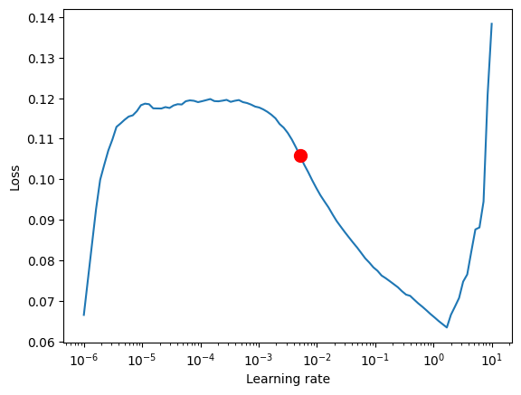
suggested learning rate: 0.011481536214968821
Train the TFT Model
These are some of the important hyperparameters for our model:
-
gradient_clip_val:hyperparameter that controls the maximum value for the norm of the gradient during training, and it can help prevent the exploding gradients problem. In this case we choose 0.447.
-
learning_rate: Learning rate determines the step size at which the optimizer travels down the loss function surface. A high learning rate can cause the optimizer to overshoot the optimal point, whereas a low learning rate can cause the optimizer to get stuck in a local minimum. A good learning rate can be found using a learning rate finder. In this case, a learning rate of 0.0051286138399136505 was chosen (via the learning rate finder).
-
hidden_size: Hidden size is the dimension of the hidden state of the LSTM. It determines the capacity of the model to store information. A larger hidden size may lead to better performance, but it also increases the risk of overfitting. In this case, a hidden size of 84 was chosen.
-
attention_head_size: Attention head size determines the number of parallel attention heads in the multi-head attention module. Increasing the number of attention heads can improve the model’s ability to learn complex temporal relationships. In this case, an attention head size of 4 was chosen.
-
dropout: Dropout is a regularization technique that randomly drops out some nodes in the network during training. It helps prevent overfitting by reducing the model’s reliance on specific nodes. A higher dropout rate means more nodes are dropped out, leading to more regularization. In this case, a dropout rate of 0.4 was chosen.
-
hidden_continuous_size: Hidden continuous size is the dimension of the hidden state of the continuous part of the model. It is set to be less than or equal to the hidden size. A smaller hidden continuous size reduces the number of parameters in the model and thus decreases the risk of overfitting. In this case, a hidden continuous size of 64 was chosen.
-
loss: The loss function is a measure of how well the model is performing. In this case, the quantile loss function was chosen. It is a robust loss function that can handle outliers and is suitable for quantile regression tasks.
-
optimizer: The optimizer determines the update rule used to update the model’s parameters based on the loss gradient. In this case, the Ranger optimizer was chosen, which combines the RAdam optimizer and LookAhead optimizer to improve convergence and generalization.
-
reduce_on_plateau_patience: This parameter determines the number of epochs to wait before reducing the learning rate when the validation loss has stopped improving. In this case, a patience of 3 was chosen.
early_stop_callback = EarlyStopping(monitor="val_loss", min_delta=1e-4, patience=40, verbose=False, mode="min")
lr_logger = LearningRateMonitor()  # log the learning rate
logger = TensorBoardLogger("lightning_logs")  # logging results to a tensorboard

trainer = pl.Trainer(
    max_epochs=100,
    #accelerator="cpu",
    accelerator="gpu",
    enable_model_summary=True,
    gradient_clip_val=0.4,
    limit_train_batches=100,  # coment in for training, running valiation every 30 batches
    # fast_dev_run=True,  # comment in to check that networkor dataset has no serious bugs
    callbacks=[lr_logger, early_stop_callback],
    logger=logger,
)


tft = TemporalFusionTransformer.from_dataset(
    training,
    learning_rate=0.03,
    hidden_size=84,
    attention_head_size=4,
    dropout=0.4, # higher dropout ~ less overfitting
    hidden_continuous_size=64,
    loss=QuantileLoss(),
    log_interval=10,  # uncomment for learning rate finder and otherwise, e.g. to 10 for logging every 10 batches
    optimizer="Ranger",
    reduce_on_plateau_patience=3,
)
print(f"Number of parameters in network: {tft.size()/1e3:.1f}k")
GPU available: True (cuda), used: True
TPU available: False, using: 0 TPU cores
IPU available: False, using: 0 IPUs
HPU available: False, using: 0 HPUs


Number of parameters in network: 897.9k
# fit network
trainer.fit(
    tft,
    train_dataloaders=train_dataloader,
    val_dataloaders=val_dataloader,
)
LOCAL_RANK: 0 - CUDA_VISIBLE_DEVICES: [0]

   | Name                               | Type                            | Params
----------------------------------------------------------------------------------------
0  | loss                               | QuantileLoss                    | 0
1  | logging_metrics                    | ModuleList                      | 0
2  | input_embeddings                   | MultiEmbedding                  | 40
3  | prescalers                         | ModuleDict                      | 2.7 K
4  | static_variable_selection          | VariableSelectionNetwork        | 60.0 K
5  | encoder_variable_selection         | VariableSelectionNetwork        | 381 K
6  | decoder_variable_selection         | VariableSelectionNetwork        | 101 K
7  | static_context_variable_selection  | GatedResidualNetwork            | 28.7 K
8  | static_context_initial_hidden_lstm | GatedResidualNetwork            | 28.7 K
9  | static_context_initial_cell_lstm   | GatedResidualNetwork            | 28.7 K
10 | static_context_enrichment          | GatedResidualNetwork            | 28.7 K
11 | lstm_encoder                       | LSTM                            | 57.1 K
12 | lstm_decoder                       | LSTM                            | 57.1 K
13 | post_lstm_gate_encoder             | GatedLinearUnit                 | 14.3 K
14 | post_lstm_add_norm_encoder         | AddNorm                         | 168
15 | static_enrichment                  | GatedResidualNetwork            | 35.8 K
16 | multihead_attn                     | InterpretableMultiHeadAttention | 17.8 K
17 | post_attn_gate_norm                | GateAddNorm                     | 14.4 K
18 | pos_wise_ff                        | GatedResidualNetwork            | 28.7 K
19 | pre_output_gate_norm               | GateAddNorm                     | 14.4 K
20 | output_layer                       | Linear                          | 595
----------------------------------------------------------------------------------------
897 K     Trainable params
0         Non-trainable params
897 K     Total params
3.592     Total estimated model params size (MB)


Sanity Checking: 0it [00:00, ?it/s]


Training: 0it [00:00, ?it/s]
best_model_path = trainer.checkpoint_callback.best_model_path
print(best_model_path)
best_tft = TemporalFusionTransformer.load_from_checkpoint(best_model_path)
lightning_logs\lightning_logs\version_129\checkpoints\epoch=67-step=1292.ckpt
# calculate baseline mean absolute error, i.e. predict next value as the last available value from the history
baseline_predictions = Baseline().predict(val_dataloader, return_y=True)
MAE()(baseline_predictions.output, baseline_predictions.y)

# calcualte mean absolute error on validation set
predictions = best_tft.predict(val_dataloader, return_y=True, trainer_kwargs=dict(accelerator="cpu"))
MAE()(predictions.output, predictions.y)

print(f'Baseline MAE: {MAE()(baseline_predictions.output, baseline_predictions.y)}, TFT MAE: {MAE()(predictions.output, predictions.y)}')
LOCAL_RANK: 0 - CUDA_VISIBLE_DEVICES: [0]


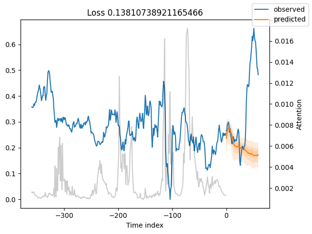
Baseline MAE: 0.1296168863773346, TFT MAE: 0.15408667922019958
# raw predictions are a dictionary from which all kind of information including quantiles can be extracted
raw_predictions = best_tft.predict(val_dataloader, mode="raw", return_x=True)
LOCAL_RANK: 0 - CUDA_VISIBLE_DEVICES: [0]
best_tft.plot_prediction(raw_predictions.x, raw_predictions.output, idx=0, add_loss_to_title=True)

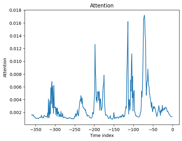
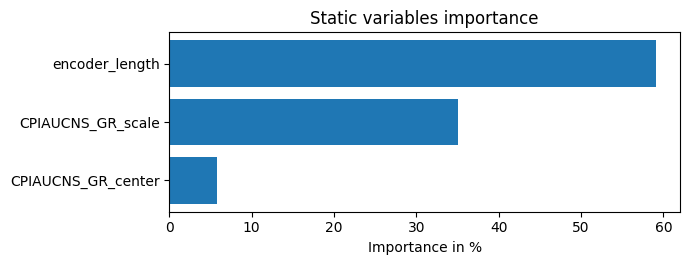
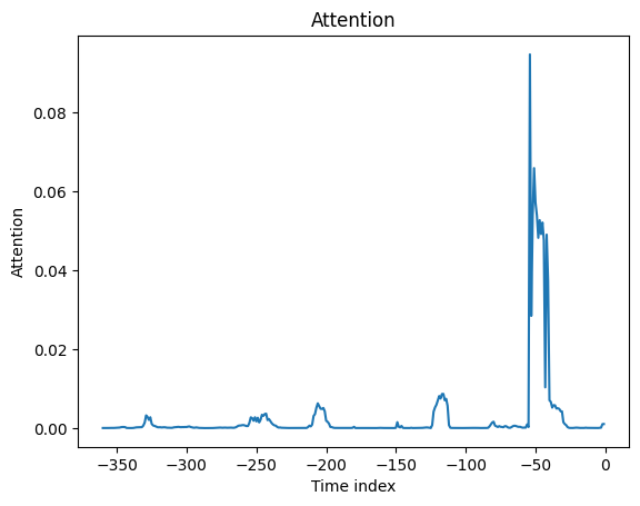
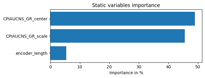
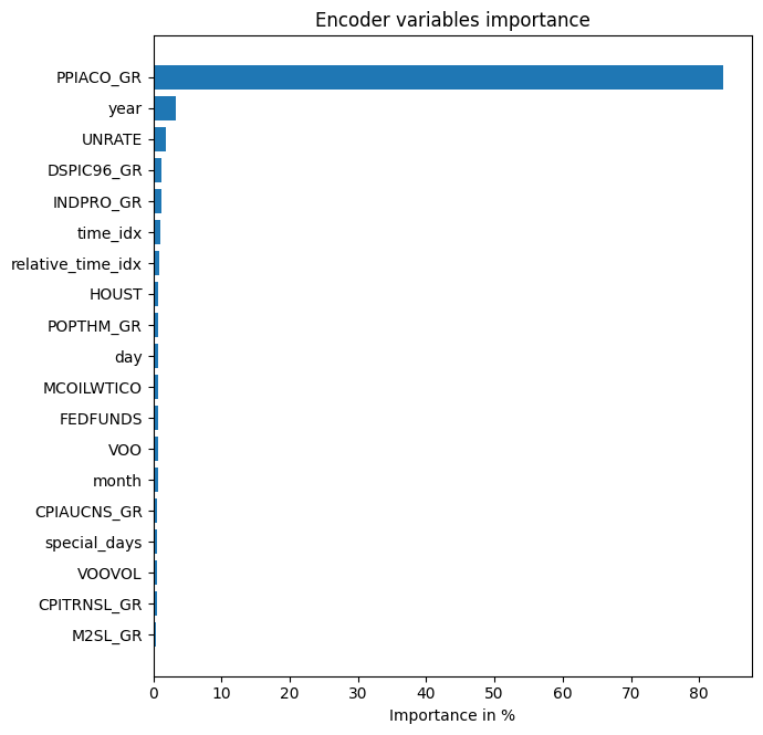
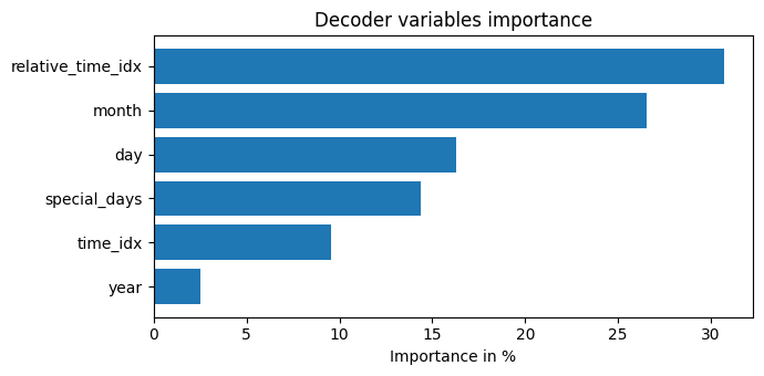
interpretation = best_tft.interpret_output(raw_predictions.output, reduction="sum")
best_tft.plot_interpretation(interpretation)
{'attention': <Figure size 640x480 with 1 Axes>,
 'static_variables': <Figure size 700x275 with 1 Axes>,
 'encoder_variables': <Figure size 700x675 with 1 Axes>,
 'decoder_variables': <Figure size 700x350 with 1 Axes>}


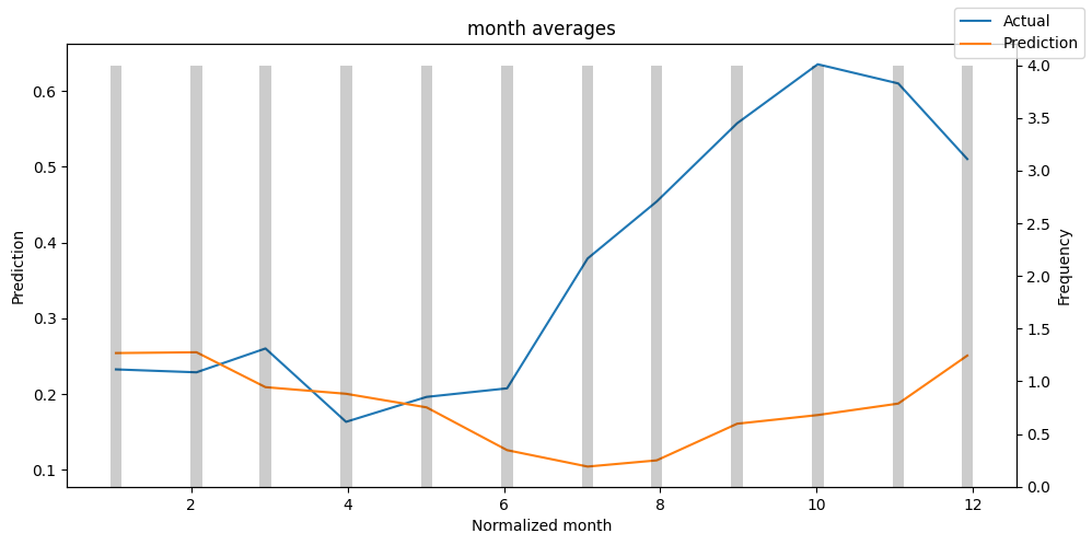
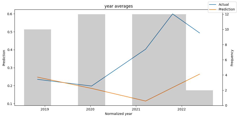
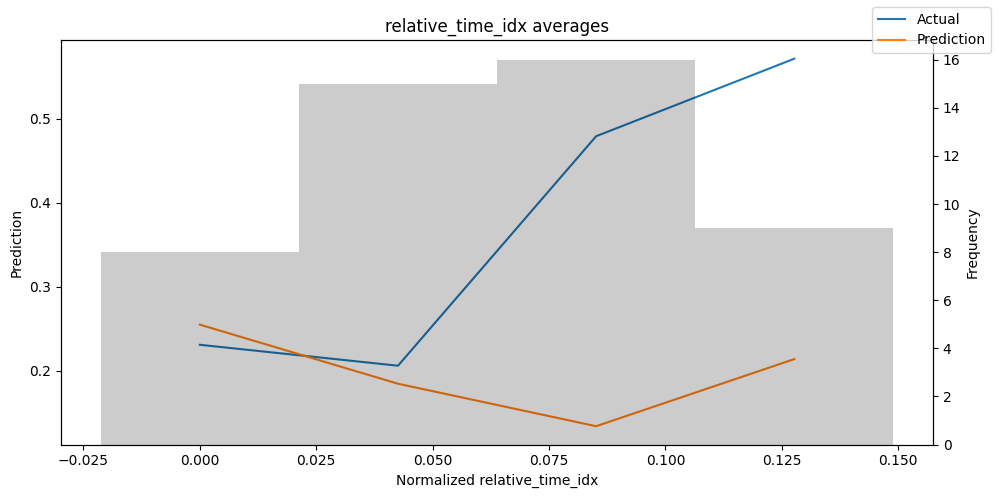
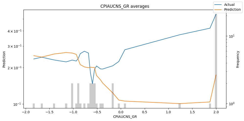
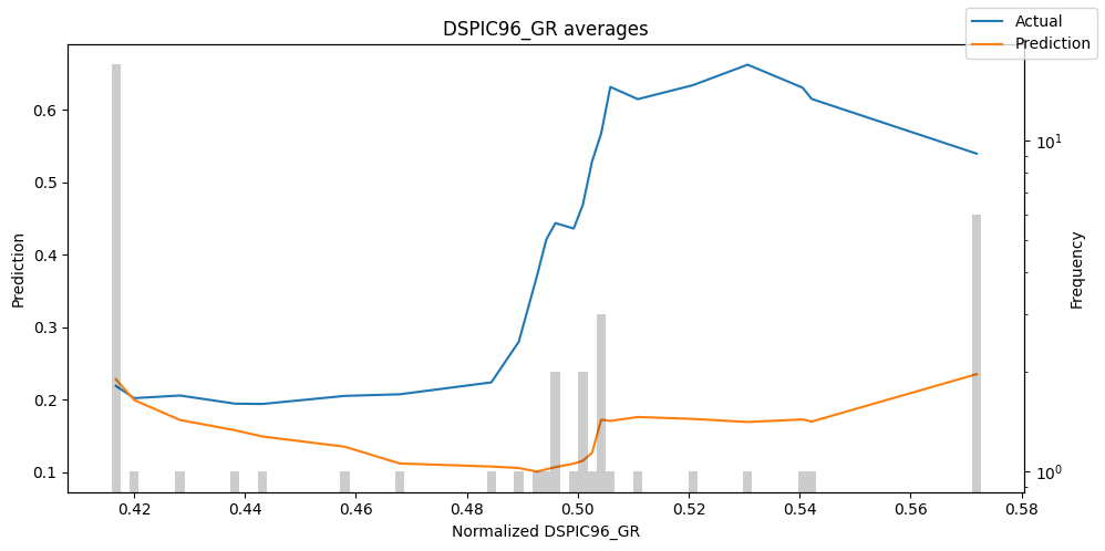
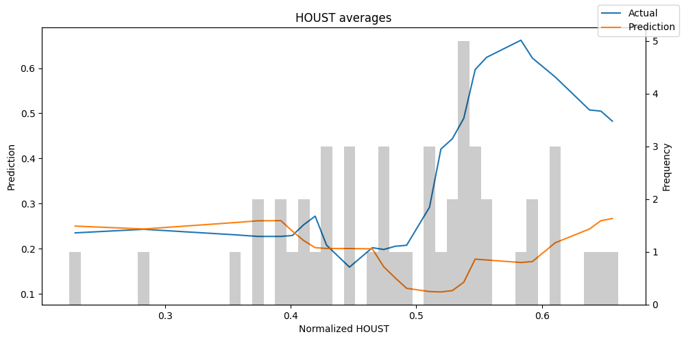
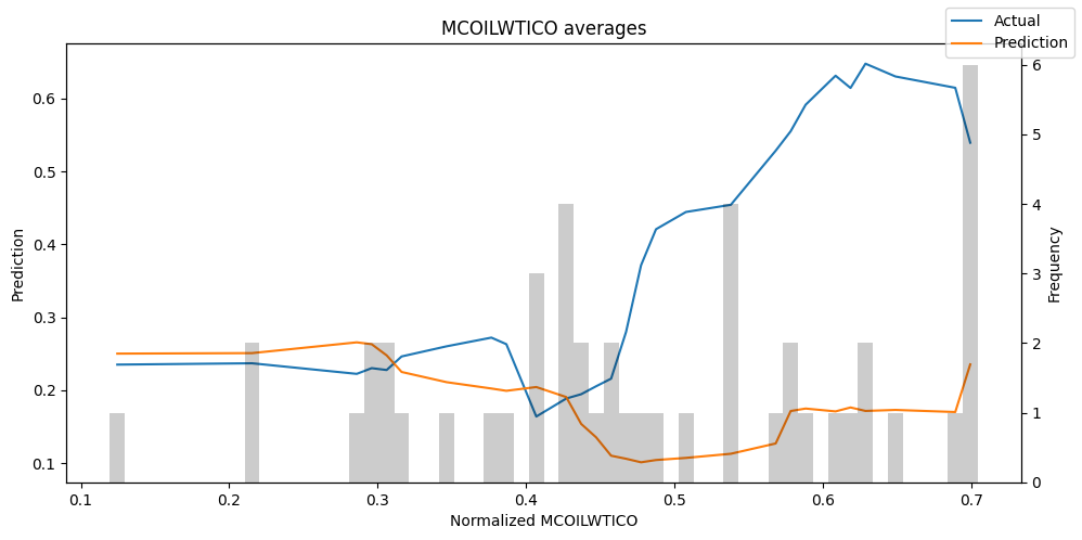
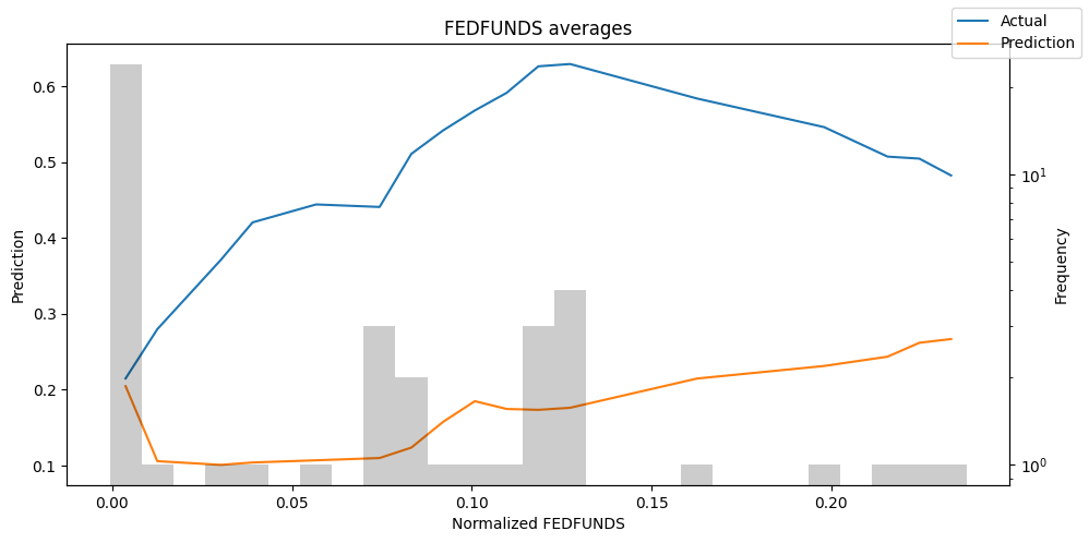
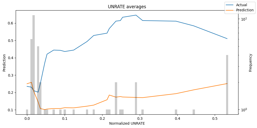
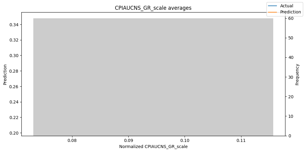
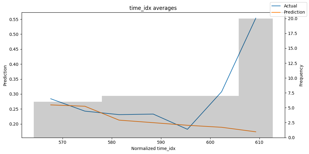
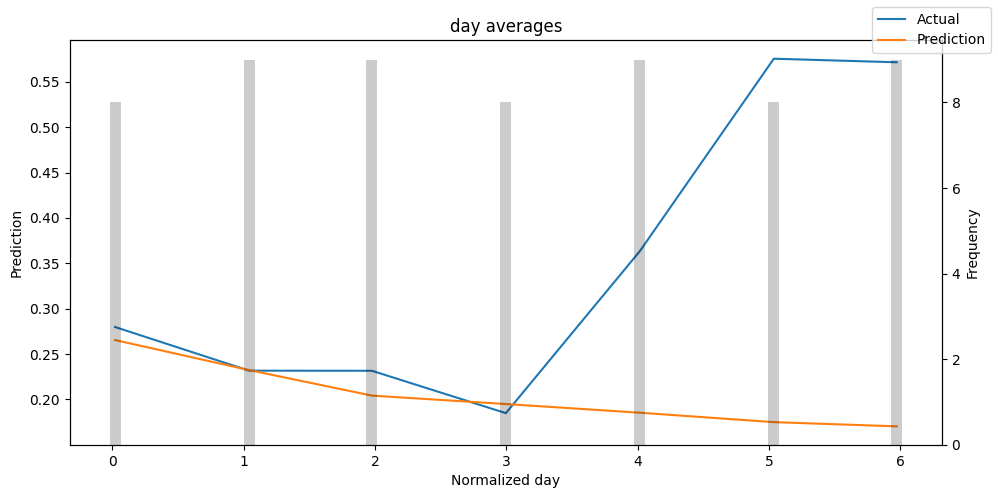
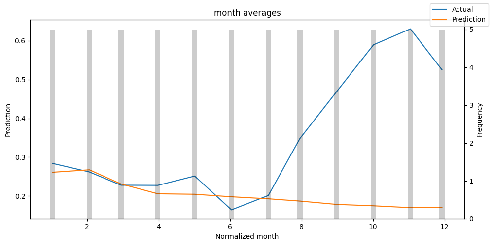
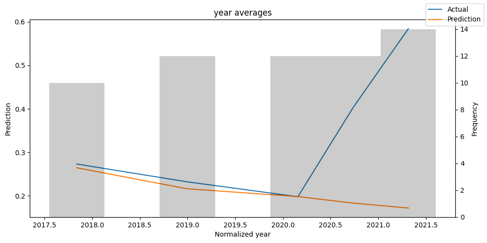
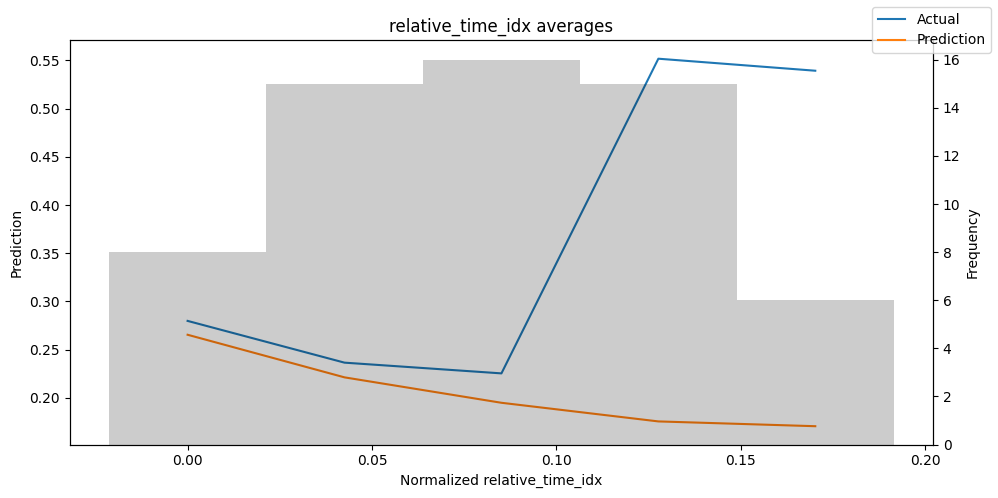
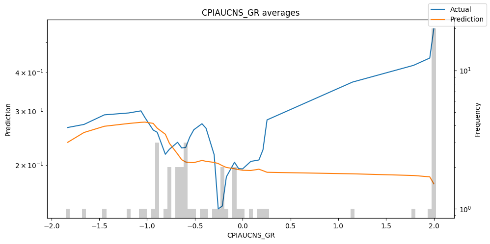
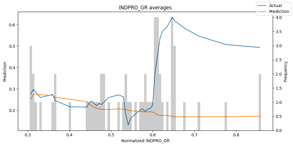
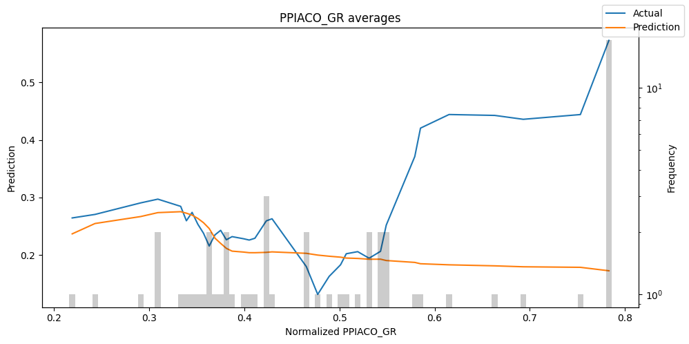
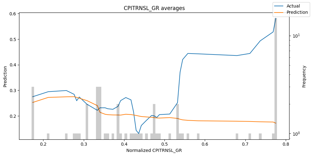
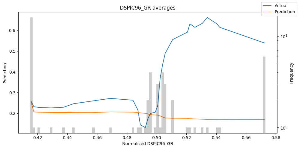
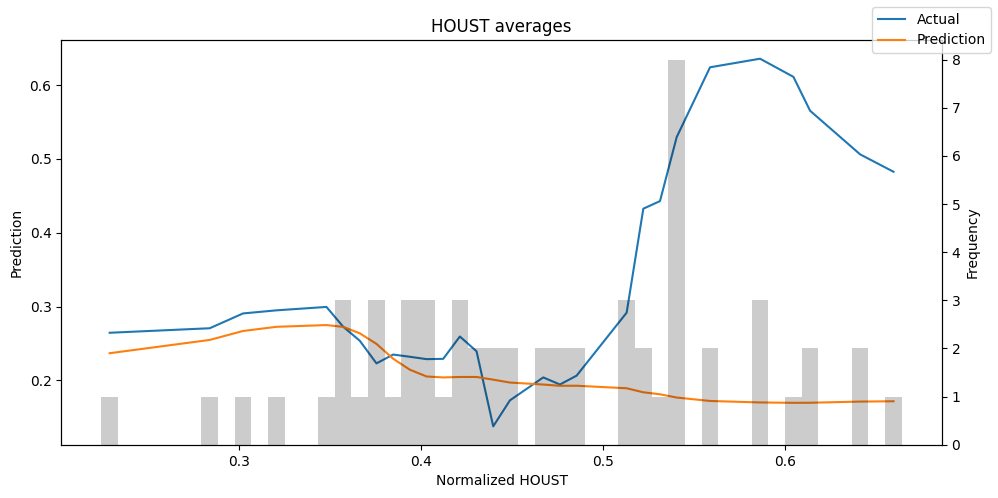
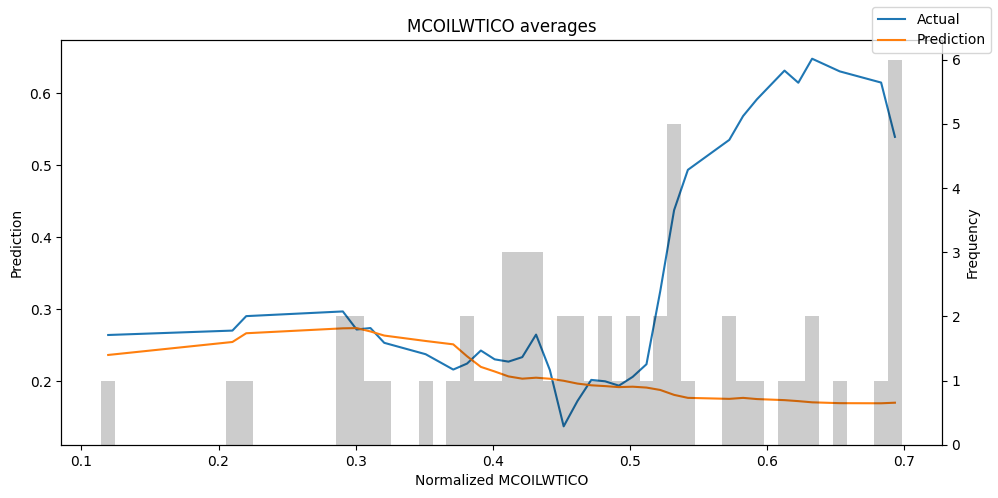
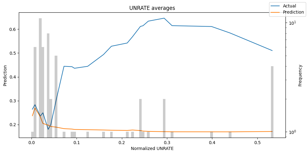
predictions = best_tft.predict(val_dataloader, return_x=True)
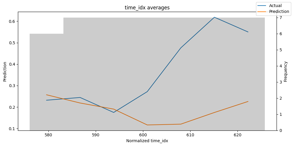
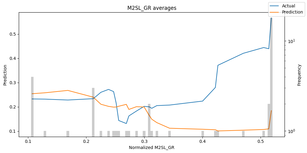
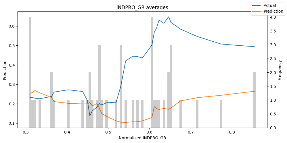
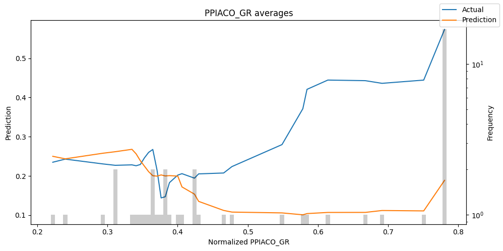
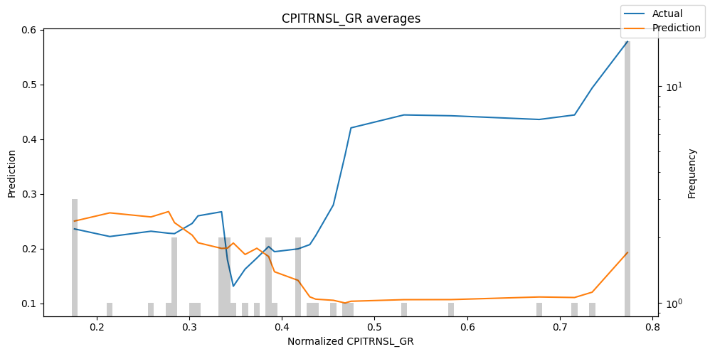
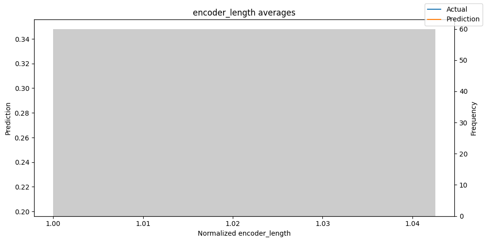
predictions_vs_actuals = best_tft.calculate_prediction_actual_by_variable(predictions.x, predictions.output)
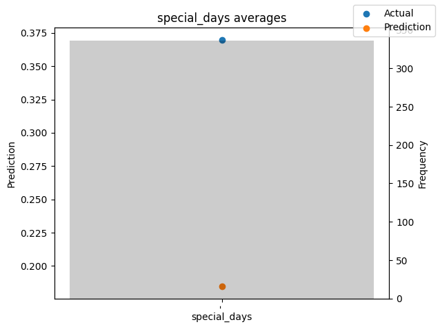
best_tft.plot_prediction_actual_by_variable(predictions_vs_actuals)
LOCAL_RANK: 0 - CUDA_VISIBLE_DEVICES: [0]






Hyperparameter Tuning With Optuna
import pickle

from pytorch_forecasting.models.temporal_fusion_transformer.tuning import optimize_hyperparameters
torch.set_float32_matmul_precision('medium')
# create study
study = optimize_hyperparameters(
    train_dataloader,
    val_dataloader,
    model_path="optuna_test",
    #n_trials=200,
    n_trials=100, # Takes to long :(
    max_epochs=100,
    gradient_clip_val_range=(0.1, 0.5),
    hidden_size_range=(32, 512),
    hidden_continuous_size_range=(16, 256),
    attention_head_size_range=(2, 8),
    learning_rate_range=(1e-5, 1e-2),
    dropout_range=(0.1, 0.5),
    trainer_kwargs=dict(limit_train_batches=40),
    reduce_on_plateau_patience=5,
    use_learning_rate_finder=False,  # use Optuna to find ideal learning rate or use in-built learning rate finder
)

# save study results - also we can resume tuning at a later point in time
with open("test_study.pkl", "wb") as fout:
    pickle.dump(study, fout)

# show best hyperparameters
print(study.best_trial.params)
[32m[I 2023-05-10 00:19:17,298][0m A new study created in memory with name: no-name-3eb3efcd-7ab1-410d-8307-9dd3c9ca1f9e[0m
GPU available: True (cuda), used: True
TPU available: False, using: 0 TPU cores
IPU available: False, using: 0 IPUs
HPU available: False, using: 0 HPUs
LOCAL_RANK: 0 - CUDA_VISIBLE_DEVICES: [0]
`Trainer.fit` stopped: `max_epochs=100` reached.
[32m[I 2023-05-10 08:10:55,623][0m Trial 41 finished with value: 0.12580467760562897 and parameters: {'gradient_clip_val': 0.2400390634531377, 'hidden_size': 47, 'dropout': 0.2501699270748916, 'hidden_continuous_size': 16, 'attention_head_size': 6, 'learning_rate': 4.676238859168727e-05}. Best is trial 20 with value: 0.11608610302209854.[0m
GPU available: True (cuda), used: True
TPU available: False, using: 0 TPU cores
IPU available: False, using: 0 IPUs
HPU available: False, using: 0 HPUs
LOCAL_RANK: 0 - CUDA_VISIBLE_DEVICES: [0]
`Trainer.fit` stopped: `max_epochs=100` reached.
[32m[I 2023-05-10 08:21:18,199][0m Trial 42 finished with value: 0.11617936193943024 and parameters: {'gradient_clip_val': 0.22077619605726787, 'hidden_size': 38, 'dropout': 0.2833960566025072, 'hidden_continuous_size': 17, 'attention_head_size': 6, 'learning_rate': 4.473341440006426e-05}. Best is trial 20 with value: 0.11608610302209854.[0m
{'gradient_clip_val': 0.44167129696837076, 'hidden_size': 50, 'dropout': 0.12768759917788702, 'hidden_continuous_size': 16, 'attention_head_size': 6, 'learning_rate': 5.688975864034011e-05}
# show best hyperparameters
print(study.best_trial.params)
{'gradient_clip_val': 0.44167129696837076, 'hidden_size': 50, 'dropout': 0.12768759917788702, 'hidden_continuous_size': 16, 'attention_head_size': 6, 'learning_rate': 5.688975864034011e-05}
# # load the best model according to the validation loss
# # (given that we use early stopping, this is not necessarily the last epoch)
# best_model_path_optuna = trainer.checkpoint_callback.best_model_path
# best_tft_optuna = TemporalFusionTransformer.load_from_checkpoint(best_model_path_optuna)
# # calculate baseline mean absolute error, i.e. predict next value as the last available value from the history
# baseline_predictions = Baseline().predict(val_dataloader, return_y=True)
# MAE()(baseline_predictions.output, baseline_predictions.y)

# # calcualte mean absolute error on validation set
# predictions = best_tft_optuna.predict(val_dataloader, return_y=True, trainer_kwargs=dict(accelerator="cpu"))
# MAE()(predictions.output, predictions.y)

# print(f'Baseline MAE: {MAE()(baseline_predictions.output, baseline_predictions.y)}, TFT MAE: {MAE()(predictions.output, predictions.y)}')
LOCAL_RANK: 0 - CUDA_VISIBLE_DEVICES: [0]


Baseline MAE: 0.1296168863773346, TFT MAE: 0.151706725358963
# #raw predictions are a dictionary from which all kind of information including quantiles can be extracted
# raw_predictions = best_tft_optuna.predict(val_dataloader, mode="raw", return_x=True)
LOCAL_RANK: 0 - CUDA_VISIBLE_DEVICES: [0]
# for idx in range(1):  # plot 10 examples
#     best_tft_optuna.plot_prediction(raw_predictions.x, raw_predictions.output, idx=idx, add_loss_to_title=True)
# interpretation = best_tft.interpret_output(raw_predictions.output, reduction="sum")
# best_tft.plot_interpretation(interpretation)
Best Model From Optuna Hyperparameter Optimization
{‘gradient_clip_val’: 0.44167129696837076, ‘hidden_size’: 50, ‘dropout’: 0.12768759917788702, ‘hidden_continuous_size’: 16, ‘attention_head_size’: 6, ‘learning_rate’: 5.688975864034011e-05}
early_stop_callback = EarlyStopping(monitor="val_loss", min_delta=1e-4, patience=40, verbose=False, mode="min")
lr_logger = LearningRateMonitor()  # log the learning rate
logger = TensorBoardLogger("lightning_logs")  # logging results to a tensorboard

trainer_optuna_results = pl.Trainer(
    max_epochs=100,
    #accelerator="cpu",
    accelerator="gpu",
    enable_model_summary=True,
    gradient_clip_val=0.2936976570290306,
    limit_train_batches=30,  # coment in for training, running valiation every 30 batches
    # fast_dev_run=True,  # comment in to check that networkor dataset has no serious bugs
    callbacks=[lr_logger, early_stop_callback],
    logger=logger,
)


tft_optuna_results = TemporalFusionTransformer.from_dataset(
    training,
    learning_rate=0.013835915722743952,
    hidden_size=73,
    attention_head_size=3,
    dropout=0.46497375562987786, # higher dropout ~ less overfitting
    hidden_continuous_size=46,
    loss=QuantileLoss(),
    log_interval=10,  # uncomment for learning rate finder and otherwise, e.g. to 10 for logging every 10 batches
    optimizer="Ranger",
    reduce_on_plateau_patience=5,
)
print(f"Number of parameters in network: {tft_optuna_results.size()/1e3:.1f}k")
GPU available: True (cuda), used: True
TPU available: False, using: 0 TPU cores
IPU available: False, using: 0 IPUs
HPU available: False, using: 0 HPUs


Number of parameters in network: 593.5k
# fit network
trainer_optuna_results.fit(
    tft_optuna_results,
    train_dataloaders=train_dataloader,
    val_dataloaders=val_dataloader,
)
LOCAL_RANK: 0 - CUDA_VISIBLE_DEVICES: [0]

   | Name                               | Type                            | Params
----------------------------------------------------------------------------------------
0  | loss                               | QuantileLoss                    | 0
1  | logging_metrics                    | ModuleList                      | 0
2  | input_embeddings                   | MultiEmbedding                  | 40
3  | prescalers                         | ModuleDict                      | 1.9 K
4  | static_variable_selection          | VariableSelectionNetwork        | 35.4 K
5  | encoder_variable_selection         | VariableSelectionNetwork        | 228 K
6  | decoder_variable_selection         | VariableSelectionNetwork        | 60.4 K
7  | static_context_variable_selection  | GatedResidualNetwork            | 21.8 K
8  | static_context_initial_hidden_lstm | GatedResidualNetwork            | 21.8 K
9  | static_context_initial_cell_lstm   | GatedResidualNetwork            | 21.8 K
10 | static_context_enrichment          | GatedResidualNetwork            | 21.8 K
11 | lstm_encoder                       | LSTM                            | 43.2 K
12 | lstm_decoder                       | LSTM                            | 43.2 K
13 | post_lstm_gate_encoder             | GatedLinearUnit                 | 10.8 K
14 | post_lstm_add_norm_encoder         | AddNorm                         | 146
15 | static_enrichment                  | GatedResidualNetwork            | 27.1 K
16 | multihead_attn                     | InterpretableMultiHeadAttention | 14.2 K
17 | post_attn_gate_norm                | GateAddNorm                     | 11.0 K
18 | pos_wise_ff                        | GatedResidualNetwork            | 21.8 K
19 | pre_output_gate_norm               | GateAddNorm                     | 11.0 K
20 | output_layer                       | Linear                          | 518
----------------------------------------------------------------------------------------
593 K     Trainable params
0         Non-trainable params
593 K     Total params
2.374     Total estimated model params size (MB)


Sanity Checking: 0it [00:00, ?it/s]


Training: 0it [00:00, ?it/s]


Validation: 0it [00:00, ?it/s]
best_model_path = trainer_optuna_results.checkpoint_callback.best_model_path
print(best_model_path)
best_tft = TemporalFusionTransformer.load_from_checkpoint(best_model_path)
lightning_logs\lightning_logs\version_126\checkpoints\epoch=48-step=931.ckpt
# calculate baseline mean absolute error, i.e. predict next value as the last available value from the history
baseline_predictions = Baseline().predict(val_dataloader, return_y=True)
MAE()(baseline_predictions.output, baseline_predictions.y)

# calcualte mean absolute error on validation set
predictions = best_tft.predict(val_dataloader, return_y=True, trainer_kwargs=dict(accelerator="cpu"))
MAE()(predictions.output, predictions.y)

print(f'Baseline MAE: {MAE()(baseline_predictions.output, baseline_predictions.y)}, TFT MAE: {MAE()(predictions.output, predictions.y)}')
LOCAL_RANK: 0 - CUDA_VISIBLE_DEVICES: [0]


Baseline MAE: 0.16816632449626923, TFT MAE: 0.20049136877059937
# raw predictions are a dictionary from which all kind of information including quantiles can be extracted
raw_predictions = best_tft.predict(val_dataloader, mode="raw", return_x=True)
LOCAL_RANK: 0 - CUDA_VISIBLE_DEVICES: [0]
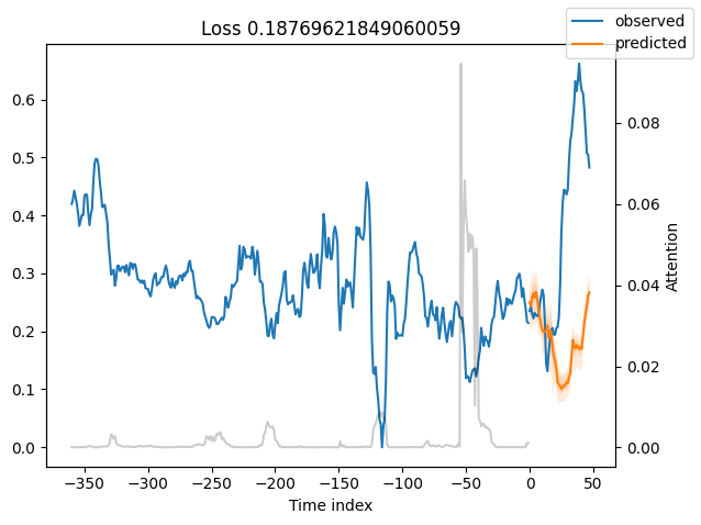
best_tft.plot_prediction(raw_predictions.x, raw_predictions.output, idx=0, add_loss_to_title=True)

interpretation = best_tft.interpret_output(raw_predictions.output, reduction="sum")
best_tft.plot_interpretation(interpretation)
{'attention': <Figure size 640x480 with 1 Axes>,
 'static_variables': <Figure size 700x275 with 1 Axes>,
 'encoder_variables': <Figure size 700x675 with 1 Axes>,
 'decoder_variables': <Figure size 700x350 with 1 Axes>}
predictions = best_tft.predict(val_dataloader, return_x=True)
predictions_vs_actuals = best_tft.calculate_prediction_actual_by_variable(predictions.x, predictions.output)
best_tft.plot_prediction_actual_by_variable(predictions_vs_actuals)
LOCAL_RANK: 0 - CUDA_VISIBLE_DEVICES: [0]
